Measuring Latency with the TSC

To find out how long it takes from receiving a market-data update to sending an order, the most direct way is to read the time at both ends and subtract. One clock_gettime call costs about 20–30 ns, yet a piece of code on a trading hot path is often only a few hundred ns, so the timing itself takes a tenth of it. That is why low-latency systems usually read the CPU’s TSC directly: one instruction, about 10 ns. Reading a hardware counter directly means answering three questions yourself: what the number stands for, whether it is read where you wrote the read, and how to turn it into nanoseconds. Part 1 covers the first two and which core a reading comes from; conversion is left to Part 2.

1. Reading the TSC: What You Read, and When

1.1 TSC (Time Stamp Counter): a Fixed-Rate Counter in Every Core

The TSC is a 64-bit counter in every logical core, cleared at power-on and counting up from then on. It has no box of its own on the hardware map; it is just a register in the core.

On early CPUs the TSC followed the core clock: it slowed down when the core slowed down and stopped in deep sleep, which made it useless for timing. Today’s CPUs have an invariant TSC: it runs at a fixed rate whether the core is throttled, asleep or in Turbo. The rate is usually close to the CPU’s nominal frequency, for example 3.593 GHz. On Linux, constant_tsc and nonstop_tsc among the flags in /proc/cpuinfo mean you have this kind.

So the TSC counts time, not the cycles the core actually ran. With the core in Turbo at 4.5 GHz and the TSC running at 3.0 GHz, 100 TSC ticks are 33 ns, during which the core ran 150 cycles. To count core cycles, use perf’s cycles event, which comes from the performance counters, not the TSC.

When the frequency changes, how the ticks change depends on what sets the time:

Pure computation: the number of cycles is set by the instructions and their dependencies and does not change with frequency. A faster core takes less time, so the TSC reads fewer ticks. Take 480 cycles: at 2.4 GHz the core takes 200 ns and a TSC running at 3.6 GHz reads 720 ticks; at 3.6 GHz it takes about 133 ns and reads 480 ticks.
Waiting on memory: the time is set by memory latency and does not change with core frequency. The ticks stay about the same, while the core idles through more cycles.
So fewer ticks don’t necessarily mean faster code; the core may just be running at a higher frequency. Before comparing two measurements, pin the frequency (turn off power saving and Turbo, or run on a core that doesn’t throttle).

Counting at 3.6 GHz, 64 bits take about 160 years to wrap, so overflow is not a concern. The cores of one CPU start counting from the same reset, so their readings are synchronized; Linux also checks at boot, and if they are not, it prints tsc: Marking TSC unstable and switches to another clock source. 1.4 relies on this.

1.2 rdtsc: 6–12 ns per Read, and on AMD the Reading Only Jumps About Every 10 ns

The most direct way to time code is to read the TSC at both ends and subtract.
Whether that difference can be trusted depends on two things: how long one read takes, and how short an interval the reading can resolve.

How to read it
- rdtsc returns the 64-bit reading in two halves: the low 32 bits in EAX, the high 32 bits in EDX. It dates from the 32-bit era, when one register couldn’t hold 64 bits.
```
inline uint64_t rdtsc() noexcept {
    unsigned int lo, hi;
    __asm__ __volatile__("rdtsc" : "=a"(lo), "=d"(hi));
    return (uint64_t(hi) << 32) | lo;
}
```
- When writing the assembly yourself, don’t drop volatile. Without it the compiler treats the asm as a computation with a fixed result and can merge two reads into one: measured, Clang 18 -O2 compiles “read twice and subtract” to returning 0.
- Prefer the compiler’s own __rdtsc() (header <x86intrin.h>): same instruction, never merged.
Why not clock_gettime
- In user space (the vDSO), clock_gettime also reads the TSC.
- But each call adds a function call and a multiply-and-shift to convert to nanoseconds: 20–30 ns per call.
- rdtsc is only the read: about 20–40 cycles, 6–12 ns.
- So on the hot path, record ticks only and convert later.
The reading moves in steps
- By frequency, one tick is 1 / 3.593 GHz ≈ 0.28 ns.
- But measured on AMD Zen parts (Ryzen, EPYC), the reading jumps only about every 10 ns, by 36 each time (36 × 0.28 ≈ 10 ns). Intel parts usually show no fixed step; back-to-back differences vary. A few back-to-back reads tell you which kind your machine is.
- Read again within the same 10 ns and you get only 1 more. That 1 is there so readings never repeat, not because 0.28 ns really passed.
- The staircase is how the counter itself updates, unrelated to how fast rdtsc reads: even if a read took no time, you’d see the same steps. 3.593 GHz ÷ 36 ≈ 100 MHz, so the reading appears to follow a roughly 100 MHz reference clock, adding 36 per tick (inferred from the numbers, not from documentation).
- Why it doesn’t step on every tick:
  - The requirement: the TSC must run at the same rate and agree across all cores, and keep running while cores slow down or sleep (1.1).
  - The core’s own clock can’t do that: it changes frequency and stops in sleep.
  - A separate 3.6 GHz clock isn’t worth it either: every core would have to keep it running all the time, which costs power, and the cores would have to agree to within 0.28 ns.
  - What is done instead: the TSC follows a slow but always-on reference clock and adds a fixed amount on every tick of it (36 here), catching up a whole tick’s worth at once.
  - Intel works the same way: its manual states in CPUID leaf 0x15 that “TSC frequency = crystal frequency × a ratio”. Intel readings show no steps, so it must subdivide between ticks; how is not published.
- Can it get finer: a single TSC read resolves one step; that is set by hardware and software can’t change it. Going finer leaves two routes:
  - Don’t rely on one read: repeat and divide, or average many runs (block 4 below); what you resolve is the average.
  - Count core cycles instead of the TSC: use the performance counter (PMU) event for unhalted core cycles, read with rdpmc, which adds 1 every cycle. The cost: the kernel must set up the counter and allow user-space reads, which virtual machines often don’t; and it counts cycles, not time, so once the core changes frequency it no longer converts to nanoseconds (1.1). This is how latencies of a few cycles per instruction get measured.
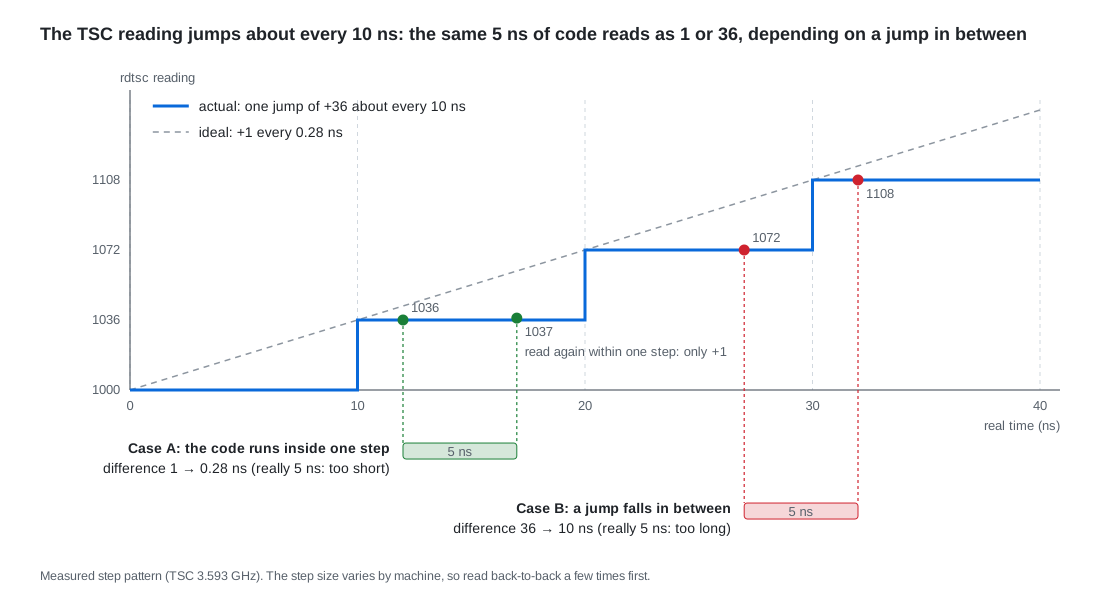
What it does to measurements
- You can’t measure rdtsc itself precisely: two back-to-back reads differ by 36 almost every time, exactly one jump, so all you can see is that a read takes at most about 10 ns.
- Any single measurement can come out only two ways: the interval crossed n jumps, or n + 1 (cases A and B in the figure). So a single measurement is off by at most one jump, about 10 ns, no matter how long the code runs. How many jumps you cross depends on where the start lands within a step, which is random, so over many runs the over- and under-counts cancel and the mean has no bias.
- What matters is how much of the measured time those 10 ns are: timing 1 µs of code, a single reading is off by at most 1%; 100 ns, by at most 10%, so one reading cannot tell 100 ns from 105 ns, and only averaging or repetition can (the two ways below); 5 ns, the error is bigger than the code itself. So don’t read single samples of code around 100 ns, and a single measurement shorter than 10–20 ns mostly reads quantization error.
- On an Intel part without steps, a single reading is not much better: without fences, out-of-order execution moves the read earlier or later by ten-odd cycles, and with fences each read gets heavier (1.3), so the edges carry about 10 ns of uncertainty anyway. About 10 ns is the resolution of a single timestamp pair, not just an AMD quirk; production marks time whole spans of hundreds of ns to several µs, where this is a few percent.
- The reading also includes the reads themselves: with nothing between two reads, the difference is still about 36. That part is roughly fixed, so measure an empty region first and subtract the floor.
- Two ways to measure short code:
  - Run it 1000 times between the two reads and divide by 1000. The error is still one jump, but per run it shrinks to about 0.01 ns.
  - Measure many times and take the mean, not the median. Where the start falls within a step is random, so 5 ns of code crosses a jump half the time, and the average comes out at (1 + 36) / 2 = 18.5 ticks ≈ 5.2 ns, close to the truth. The median gets pulled to one of the two outcomes: 3 ns of code crosses a jump only 30% of the time, so the median is 1 tick, read as 0.28 ns.
- This is how benchmarks report differences like 52.6 ns vs 52.5 ns: the first way above. The tool (Google Benchmark, say) loops the code hundreds of thousands to millions of times and divides the total by the count, so one jump of error shrinks to around a hundred-thousandth of a ns per run. What limits the result then is run-to-run variation (frequency, caches, code alignment), not timer resolution; whether a 0.1 ns difference is real takes several runs and a check that the intervals don’t overlap.
- Save medians and percentiles such as p99 for intervals much longer than a jump, such as a full processing path of hundreds of ns to a few µs, where quantization is a few percent.
- Errors from out-of-order execution are a separate matter; see 1.3.

1.3 Out-of-Order Execution: rdtsc Doesn’t Wait for Earlier Instructions

Why the edges are fuzzy
- Out-of-order execution: the CPU does not finish instructions one by one in program order (the “Rename + ROB” box on the hardware map). rdtsc reads without waiting for the instructions before it to finish, and instructions after it may start before it.
- With just two reads and a subtraction, look at this:
```
uint64_t t0 = __rdtsc();
int r = parse(msg);        // the code being measured
uint64_t t1 = __rdtsc();
```
- Start: the first few instructions of parse may begin before t0 is read.
- End: when t1 is read, the last few instructions of parse may not have finished.
- Result: both edges move inward, so when the measured code is only tens of ns, the measurement comes out shorter than the real one.
The fix: pin the edges with fences
- lfence: the instructions after it may not start until all the instructions before it have finished.
- rdtscp: a variant of rdtsc that waits for all earlier instructions to execute and all earlier loads to complete before reading, but does not hold back later instructions.
- The start and end marks look like this:
```
inline uint64_t tsc_begin() {      // start mark: read only after earlier instructions finish
    _mm_lfence();
    uint64_t t = __rdtsc();
    _mm_lfence();                  // later instructions may not start early
    return t;
}

inline uint64_t tsc_end() {        // end mark: rdtscp waits for earlier instructions before reading
    unsigned aux;
    uint64_t t = __rdtscp(&aux);
    _mm_lfence();                  // later instructions may not start early
    return t;
}
```
- Start mark: the first lfence lets the earlier code finish; the second keeps the measured code from starting before the read.
- End mark: rdtscp waits for the measured code to finish before reading; the lfence after it keeps later code from starting early.
- rdtscp only covers the front: it waits for earlier instructions before reading, but does not hold back later ones, so the code after it may start executing before it reads. That is why it still needs an lfence after it.
- When that second fence matters: with back-to-back marks, one reading is both the end of one span and the start of the next (t0, t1, t2 read in turn), so both sides must be pinned. When you time a single span and nothing after it is measured, it makes little difference, but it costs nothing to keep the same form everywhere.
- The start mark can use rdtscp too: replacing the leading lfence + rdtsc with a single rdtscp does the same thing, waiting for earlier instructions before reading, and the lfence after it is still needed. The bonus is that you get aux and can catch migrations (the code in 1.4 does exactly this).
Intel vs. AMD
- Intel: this behavior of lfence is defined in the manual.
- AMD: lfence only waits like this once the operating system turns on a switch. Recent Linux and Windows do so by default; on older systems AMD recommends mfence.
- If earlier stores must also be visible to other cores: the sequence Intel’s manual gives is mfence; lfence; rdtsc.
What fences cost, and when to use them
- Extra overhead: measured on an empty interval, the difference between two fenced reads goes from one jump to two, about 20 ns, one jump more than without fences.
- No more overlap: fences stop the measured code from overlapping with the code around it, so what you measure is no longer exactly how it normally runs.
- Fences make the edges accurate, at the cost of a heavier measurement and code that no longer overlaps with its neighbors.
- Which to use:
  - Microbenchmarks: for code of tens of ns, the edge error is as large as the code itself, so use fences.
  - Production hot path: marks there measure whole spans of several µs, where an edge error of ten-odd ns is acceptable, so a plain rdtsc is the usual choice.
The compiler moves code too
- Deleted entirely: if nothing uses the result of the measured code, the compiler may remove it.
- Moved outside: computations that don’t touch memory may be moved outside the two reads.
- Fix: make sure the result is used, for example by writing it to a volatile variable.

1.4 rdtscp and Cores: Knowing Which Core You Read On

aux: which core you read on, for free
- What it reads: besides the TSC, rdtscp reads the IA32_TSC_AUX register into ECX, which is the aux in the code above.
- What’s in it: Linux sets this register on each core to “NUMA node × 4096 + core number”, and getcpu in the vDSO relies on it. Split apart:
```
unsigned core = aux & 0xfff;   // low 12 bits: core number
unsigned node = aux >> 12;     // the rest: NUMA node
```
Catching migrations: drop the sample if the two aux differ
- How: use rdtscp at both start and end, and compare the two aux values. tsc_begin in 1.3 uses rdtsc, which gives no aux, so when you want to catch migrations, switch the start read to rdtscp too:
```
unsigned a0, a1;
uint64_t t0 = __rdtscp(&a0);   // start: rdtscp itself waits for earlier code
_mm_lfence();                  // measured code may not start early
int r = parse(msg);
uint64_t t1 = __rdtscp(&a1);   // end
_mm_lfence();
bool migrated = (a0 != a1);    // moved to another core in between
```
- What a difference means: the thread was moved to another core in between, so the span includes a migration (#1 1.1), and the two cores’ readings may not line up exactly.
- What to do: throw the sample away, or mark it separately.
- Hot threads: pinned to one core as in #1, they never hit this.
Subtracting across cores: fine on one machine
- The case: a producer on core 2 stamps a message as it writes it into a queue, the consumer on core 4 stamps it again when it takes it out, and the difference is how long the message sat in the queue.
- Why it works: as 1.1 said, the cores of one machine have synchronized TSCs.
- Watch out: the sync is not perfect. When the queueing time is very short, the difference can be a tiny negative number. That means the queueing time is within the sync error, not that the program is broken.
When you can’t subtract: the sync assumption breaks
- The assumption: subtracting across cores works only because the cores’ TSCs are synchronized (1.1). In the cases below, that assumption fails.
- The TSC on this machine isn’t synchronized: firmware (BIOS) wrote the TSC, or the sockets of a multi-socket server aren’t aligned. Linux catches this at boot and prints tsc: Marking TSC unstable (1.1), visible in dmesg; then cross-core differences can’t be trusted.
- Virtual machines: the hypervisor may add an offset to the TSC, or skew it when a virtual CPU moves to another physical core, so subtracting across cores is no longer reliable.
- Two machines: they don’t share a counter at all, so there is nothing to synchronize and nothing to subtract. To line up times across machines, use the PTP-synchronized system clock (1.5, block 4).
Checking that a machine supports this
- CPUID: bit 27 of EDX in leaf 0x80000001 is rdtscp, and bit 8 of EDX in leaf 0x80000007 is invariant TSC.
- On Linux it’s easier: check /proc/cpuinfo for these three flags.
```
grep -o 'rdtscp\|constant_tsc\|nonstop_tsc' /proc/cpuinfo | sort -u
```

1.5 Marks on the Hot Path: Record Ticks, Leave Conversion and Output to Another Thread

A mark costs time too
- Where it goes: about 10 ns to read the TSC, plus a memory write or an enqueue to record it.
- The hot path does only those two steps: store the difference in ticks into a preallocated array, or hand it to the asynchronous logger of #4.
- Everything else moves away: conversion to nanoseconds, formatting and file writes all happen on another thread.
A common form: a pair of macros
```
#define START_MEASURE(TAG) const auto TAG = Common::rdtsc()

#define END_MEASURE(TAG, LOGGER)                       \
    do {                                               \
        const auto end = Common::rdtsc();              \
        LOGGER.log("RDTSC " #TAG " %\n", (end - TAG)); \
    } while (false)
```
- START_MEASURE: reads the TSC once into a local variable named TAG.
- END_MEASURE: reads it again and hands the difference to the logger.
- LOGGER.log: only puts its arguments into a lock-free queue; the logger thread formats them later.
- Units: the end - TAG in the log is a tick count, not nanoseconds.
- Don’t build a time string here: calling a “current time as a string” function inside END_MEASURE puts formatting right back on the hot path. If you want a time, record the raw number and let the logger thread convert it.
- Cost: every mark adds tens of ns to the hot path, so in production mark only a few key points, or sample.
Across threads and machines: record absolute timestamps
- What a TSC span can’t cover: it suits a piece of code within one thread. A trade goes from the market-data thread to the strategy thread to the order thread, often across processes, from receiving the update to sending the order.
- How: every stage records an absolute timestamp, and afterwards the records of each stage are joined per order, which shows how long each leg took. This kind of record is called tick-to-trade (TTT):
```
#define TTT_MEASURE(TAG, LOGGER)                    \
    do {                                            \
        const auto TAG = Common::getCurrentNanos(); \
        LOGGER.log("TTT " #TAG " %\n", TAG);        \
    } while (false)
```
- getCurrentNanos(): returns nanoseconds since 1970, i.e. the system clock.
TSC or system clock
- Several processes on one machine: they could in fact share the TSC, since the cores’ TSCs are synchronized (1.1).
- Lining up with exchange reports or other machines: the TSC can’t do that; you need the system clock that every machine has synchronized (via PTP).
- Use the TSC for spans within one thread, and a shared absolute clock to build timelines across components and machines.
Look at the distribution, not one run
- One measurement means little: the same code takes 300 ns one time and 2 µs the next when it hits a cache miss.
- What matters: the distribution over many measurements, i.e. the median, the 99th percentile, the maximum. That is the subject of the next item, measuring trading-system performance.

2. Conversion and Calibration: Turning Ticks into ns

Everything recorded in part 1 is in ticks. Turning them into ns requires knowing how many ticks the TSC advances per second: the TSC frequency.
Get that number wrong and every time is wrong by the same ratio, with nothing to show for it. So first the conversion itself, then where the frequency comes from, how to measure it yourself, and where the measurement belongs.

2.1 Conversion: Divide Ticks by the TSC Frequency

The formula
$$t_{\text{ns}} = \frac{\Delta \text{tick}}{f_{\text{TSC}}} \times 10^9$$
- Only one number is missing: you already have the difference $\Delta \text{tick}$; what’s missing is the TSC frequency $f_{\text{TSC}}$.
- Whatever the frequency is off by, every time is off by: compute with 3.0 GHz when the real value is 3.593 GHz and every time comes out about 20% too long (3.593 ÷ 3.0 ≈ 1.198). Nothing reports an error; the numbers still look plausible.
- Where to compute it: the hot path records only ticks (1.5); convert on the logger thread or afterwards.
Integer multiply-then-divide overflows
- The usual form: ticks * 1000000000ULL / freq, multiplying by $10^9$ first to keep precision.
- Where it overflows: the product must fit in 64 bits, so $\Delta \text{tick}$ can be at most about $1.8 \times 10^{10}$ ($2^{64} \div 10^9$). At 3.6 GHz, any span over about 5 seconds overflows, giving an absurdly small number, again without any error.
- Fix: compute in double, whose 15–16 significant digits are plenty at ns scale; or precompute ns_per_tick = 1e9 / freq and multiply once per conversion.

2.2 Where the Frequency Comes From: Look It Up, Measure Only if You Can’t

The kernel measured it at boot
- Where to look: dmesg | grep -i tsc shows a line like tsc: Refined TSC clocksource calibration: … MHz or tsc: Detected … MHz processor.
- How it got there: at boot the kernel timed the TSC against another clock (HPET, PIT and the like).
- How to use it: read it once at deployment and put it in the config.
Intel: CPUID leaf 0x15
- What it gives: the crystal frequency (ECX) and a ratio (EBX ÷ EAX). TSC frequency = crystal frequency × ratio, the “slow crystal plus a fixed amount per tick” from 1.2, block 3.
- It may be empty: some models report ECX as 0, leaving out the crystal frequency; in a virtual machine the whole leaf may be 0 (measured on a cloud Intel VM: leaves 0x15 and 0x16 both return 0).
```
uint64_t freq_from_cpuid_15() {
    unsigned eax, ebx, ecx, edx;
    if (!__get_cpuid(0x15, &eax, &ebx, &ecx, &edx)) return 0;   // leaf doesn't exist (most AMD)
    if (eax == 0 || ebx == 0 || ecx == 0) return 0;              // ratio or crystal not reported (common in VMs)
    return uint64_t(ecx) * ebx / eax;
}
```
- __get_cpuid: checks first that the leaf exists and returns 0 if not, so you never read garbage.
- Return 0 when unknown: let the caller know to try something else, instead of falling back to a hard-coded default.
Don’t use CPUID leaf 0x16
- What it is: the processor’s nominal base frequency in MHz, meant for humans; Intel does not promise it equals the TSC frequency.
- AMD doesn’t have it: AMD does not define this leaf, so the query fails.
- The consequence: use it as the TSC frequency and fall back to 3.0 GHz when it’s missing, and on a 3.593 GHz machine every time comes out about 20% too long.
If none of that works, measure it yourself: calibrate against steady_clock, see 2.3.

2.3 Calibrating It Yourself: Time a Span Against steady_clock

How
- Record a pair at each end: at the start, record a TSC reading and the steady_clock time; wait for a span $T$; record another pair at the end.
- Compute the frequency:
$$f_{\text{TSC}} = \frac{\text{tick}_1 - \text{tick}_0}{t_1 - t_0}$$
Where the error comes from: the pairing error at each end
- Pairing error: the TSC and steady_clock are not read at the same instant; one now() call sits between them (20–30 ns, 1.2), and occasionally an interruption. Call it $\delta$.
- Spread over the baseline: each end has its own $\delta$, so the relative error in the frequency is about
$$\frac{\Delta f}{f} \approx \frac{\delta_0 + \delta_1}{T}$$
- Example: 60 ns in total over a 100 ms baseline gives $60 \div 10^8 = 6 \times 10^{-7}$, i.e. 0.6 ppm. Converting a 1 ms span with that frequency is off by only 0.6 ns.
- So a longer baseline is more accurate. With a baseline on the order of 100 ms, the error is already far below one step from 1.2 (about 10 ns).

Shrinking the pairing error: sandwich one now() between two TSC reads

tsc_arr[0] = rdtsc();
for (int i = 0; i < try_times; ++i) {          // try_times = 5
    ns_arr[i] = std::chrono::steady_clock::now();
    tsc_arr[i + 1] = rdtsc();
}

auto min_tsc_diff = tsc_arr[1] - tsc_arr[0];
auto ave_tsc = average(tsc_arr[0], tsc_arr[1]);
auto ns = ns_arr[0];
for (int i = 1; i < try_times; ++i) {
    auto tsc_diff = tsc_arr[i + 1] - tsc_arr[i];
    if (tsc_diff < min_tsc_diff) {               // keep the tightest sandwich
        min_tsc_diff = tsc_diff;
        ave_tsc = average(tsc_arr[i], tsc_arr[i + 1]);
        ns = ns_arr[i];
    }
}
return {ave_tsc, ns};

Sandwiching: the instant now() read must fall between the two rdtsc around it. Taking the midpoint of the two readings as the paired TSC value, the error is at most half the gap.
Five tries, keep the tightest: the smallest gap means nothing interrupted or rescheduled the thread in between.
How wide the gap is: one now() plus one rdtsc, about 30–40 ns at the tightest, so the midpoint is off by under 20 ns.

Which clock to calibrate against
- steady_clock: monotonic, never jumps back (CLOCK_MONOTONIC on Linux).
- system_clock jumps: NTP corrections or someone setting the time move it forward or back in one step. A jump during the 100 ms calibration makes the frequency wrong.
- Avoid high_resolution_clock: in libstdc++ (GCC’s default standard library) it is system_clock (measured: std::is_same is true); in libc++ it is steady_clock. The same line of code means different things under different standard libraries.
- Cleaner still: NTP also slews the rate of steady_clock, adjusting speed without jumping. To avoid even that, use clock_gettime(CLOCK_MONOTONIC_RAW, …).

2.4 Two Timers: When to Calibrate

TSCTimer: calibrate on the first read of a result
- One pair at startup: base_point is a static variable, so at program start it records a (TSC, steady_clock) pair with the sandwich from 2.3.
- Another pair on the first get(): subtracting the two pairs gives cycle_to_ns_scale (ns per tick), stored in an atomic and never recomputed.
```
static void calibrate() {
    auto [end_tsc, end_time] = TimerHelper::get_tsc_ns_pair();
    auto& [begin_tsc, begin_time] = TimerHelper::base_point;
    std::chrono::nanoseconds duration = end_time - begin_time;
    auto scale = static_cast<double>(duration.count()) / static_cast<double>(end_tsc - begin_tsc);
    double expected = 0.;
    cycle_to_ns_scale.compare_exchange_strong(expected, scale, std::memory_order_relaxed);
}
```
- compare_exchange_strong: if several threads call get() for the first time at once, only the first write counts and the rest use its result.
- The upside: start / end only read the TSC and never touch another clock; the baseline is “program start to first get()”, usually long, so the error is small.
- The cost: the first get() makes 5 now() calls, about 100–150 ns, a spike if it lands on the hot path. Call get() right after startup and the baseline is too short as well.
- How to use it: during startup, wait a while (say 100 ms or more) and call get() once yourself, so calibration happens off the hot path.
TSCTimer: one reading ends one span and starts the next
```
timer.start(1);
some_work(20);
timer.start(0, timer.stop, 1);   // one reading: start span 0, end span 1
some_work(30);
timer.end(0);
```
- Accumulation: each span has a slot; end does cycles_arr_[i] += tsc - last_tsc_arr_[i], so repeated measurements of the same span add up.
- Switching with one reading: this is the back-to-back marking from 1.3: one reading is both the end of span 1 and the start of span 0. One read fewer, and no gap between the two spans.
- No fences: start / end contain only rdtsc or rdtscp, fine for ms-scale spans; for code of tens of ns, add lfence as in 1.3.

HardwareTimer: calibrated in the constructor

Done at construction: it first uses CPUID to check for the TSC, rdtscp and invariant TSC, then calibrates 5 times at 100 ms each and takes the median. Construction takes over 0.5 seconds, so it belongs in startup.
Each calibration checks for migration: rdtscp at both ends, and if aux differs, redo it (1.4).
The median: if one or two of the five runs are interrupted, the median is unaffected.
One calibration run can be written like this:

// time a baseline against steady_clock, return the TSC frequency (Hz); 0 if every one of max_retry tries switched cores
double calibrate(std::chrono::milliseconds baseline, int max_retry = 5) {
    using clock = std::chrono::steady_clock;
    for (int attempt = 0; attempt < max_retry; ++attempt) {
        unsigned a0, a1;
        auto c0 = clock::now();
        uint64_t t0 = __rdtscp(&a0);
        std::this_thread::sleep_for(baseline);
        uint64_t t1 = __rdtscp(&a1);
        auto c1 = clock::now();
        if (a0 != a1) continue;                          // switched cores: discard and retry
        double ns = std::chrono::duration<double, std::nano>(c1 - c0).count();
        return double(t1 - t0) * 1e9 / ns;               // in double: no overflow
    }
    return 0;                                            // keeps switching cores: pin first, then calibrate
}

Against steady_clock: for the reasons in 2.3, block 4.
In double: avoids the integer overflow from 2.1.
Bounded retries: an unpinned thread on a busy machine may keep being moved, and unbounded retries would spin forever. After a few tries return 0 and let the caller pin the thread (#1) and calibrate again.
Fail loudly when the frequency is unknown: per 2.2, don’t fall back to a hard-coded default.

Which to pick
- TSCTimer: calibrates late and costs little, good for timing a few spans anywhere in the program.
- HardwareTimer: pays 0.5 seconds at startup for a calibration you can check (migration, median), good when you want to confirm the machine and frequency before starting.
- Both keep calibration off the hot path; on the hot path there is only a TSC read.

2.5 The TSC in a Virtual Machine

The readings are altered
- Offset: the hypervisor adds an offset to each VM’s TSC so it appears to start when the VM booted.
- Scaling: when a VM migrates to a physical machine with a different TSC frequency, readings must be scaled. With TSC scaling support in the CPU, hardware does it; without it, rdtsc has to be trapped and emulated, and every read goes in and out of the VM, slowing to the µs range.
The frequency is hard to get
- CPUID may be all zeros: neither 0x15 nor 0x16 answers (2.2).
- The kernel knows: the guest kernel gets the frequency from the hypervisor, and dmesg still shows tsc: Detected … MHz.
- So in a VM: take the kernel’s value first, then measure it yourself as in 2.3 to cross-check.
The clock source may be swapped
- Where to look: cat /sys/devices/system/clocksource/clocksource0/current_clocksource; VMs commonly show tsc or kvm-clock.
- When the TSC is judged unreliable: the kernel falls back to a clock source like HPET, and every clock_gettime has to go to the chipset, rising from 20–30 ns to about 0.5–1.5 µs (#19 4.1).
- tsc=reliable: makes the kernel skip its checks on the TSC, so one hiccup can’t disqualify it (#19 4.2). Add it only when you’re sure the TSC is sound.
- Effect on calibration: rdtsc still works; what changes is steady_clock: the reference clock now takes µs per read, the pairing error grows with it, and the baseline has to grow accordingly.