
Saying a trading system has “3 µs latency” carries no information by itself. 3 µs from where to where? Mean or 99th percentile? Measured while idle, or during the burst at the open? Without those answers two systems’ numbers can’t be compared, and after a round of optimization you can’t tell which leg the saved time came from. So the first thing is to say which leg you are measuring.
1. What to Measure, How to Report It, Where to Mark
1.1 Latency Metrics: Which Leg TTT and RTT Each Cover
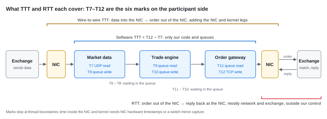
TTT (tick-to-trade): from receiving market data to sending the order
- What it covers: everything between a market-data update arriving and the order it triggers leaving the system: parsing, updating the book, computing the signal, risk checks, sending.
- Why it matters most: this leg is all our own code and machines, the part we can optimize. High-frequency trading competes on exactly this leg.
- Software TTT: marks inside the threads, T12 − T7 (how to write the marks is in #20 1.5). It only reaches the thread boundaries: the time the data spends in the NIC and kernel, and the time from
senduntil the order actually leaves the NIC, are not in it. - Wire-to-wire TTT: from data entering the NIC to the order leaving the NIC. It needs hardware timestamps taken by the NIC, or a mirror of the traffic at the switch, timestamped by a capture appliance on one clock. When the industry quotes TTT, this is usually what it means.
- Both need only two times, one at each end: software TTT uses just T7 and T12; T8–T11 in between are for splitting it into legs (1.3). Wire-to-wire TTT is also two times, just taken outside the software. Both need pairing per message: in software, the message ID brings T7 and T12 together; a capture appliance only sees packets, so it pairs the sequence number in the market-data packet with the order ID in the order packet, using the program’s own log of “this sequence number triggered this order”.
- The difference between them: exactly the NIC and kernel legs. With kernel bypass (reading packets straight from the NIC, skipping the kernel’s network stack) those legs get much shorter, but not zero.
RTT (round-trip time): from the order going out to the reply coming back
- What it covers: the order leaving the NIC, crossing the network to the exchange, being matched, and the reply coming back.
- Mostly outside our control: network distance and exchange processing are in it. It’s for watching whether the network or the exchange got slower, not for optimizing our own code.
TTFB (time to first byte)
- What it is: from sending a request to receiving the first byte of the response, common for web and network services.
- Rarely used in trading systems: market data is pushed, not requested, and TTT and RTT already split the two legs worth measuring.
1.2 Statistical Metrics: Look at the Distribution, Not the Mean
The mean hides spikes
- Why: latency distributions are skewed. Most samples sit in a narrow band, and a few interrupted ones drag out a long tail. The mean only reflects the total; it can’t tell you how long the tail is.
- A constructed example: one million samples, 99.8% between 280 and 320 ns, 0.2% being 20 µs spikes:
mean p50 p99 p999 max 339 ns 310 ns 330 ns 20 µs 20 µs - How to read it: the mean is only 10% above p50 and p99 looks great, yet one update in every 500 waits 20 µs, and only p999 and the max show it.
Which numbers to report
- p50 (median): half the samples are faster; this is the usual case.
- p99, p999: roughly how slow the slowest one in 100 or in 1000 is, i.e. the tail latency.
- max: the single worst case, often a thread being switched out, a page fault and the like (the “system” group of the reference table 2.1).
- Jitter: variance alone isn’t enough because the distribution is so skewed. p99 − p50 or p999 − p50 is the usual way to state how large the jitter is.
- Plus two conditions: how many samples, and under what load. Without those, percentiles can’t be compared with anyone else’s.
Why the tail matters
- Spikes aren’t spread evenly: when market data is densest (the open, large orders, news), queues back up most easily, caches get flushed most easily, and latency spikes most easily.
- That’s also when the opportunities are: the few hundred updates where prices move fastest and matter most land precisely in the tail. So a trading system has to push down tail latency, not average latency.
You need enough samples
- p999 means seeing the slowest one in a thousand: 10,000 samples leave only 10 above p999; with fewer, you’re guessing.
- Rule of thumb: to estimate the $1 - 1/k$ quantile you need at least tens of times $k$ samples; tens of thousands for p999, hundreds of thousands for p9999.
Computing percentiles in production: a histogram
- You can’t sort every time: millions of samples a day make sorting expensive, and it doesn’t belong on the hot path.
- A fixed-width histogram: add one to the bucket a latency falls into; to get a percentile, accumulate from the smallest bucket up to the one holding sample number $p \times \text{total}$:
// fixed-width latency histogram: one division and one increment per sample struct LatencyHist { static constexpr uint64_t kBucketNs = 10; // 10 ns per bucket static constexpr size_t kBuckets = 10000; // 0–100 µs; everything above goes into the last bucket std::array<uint64_t, kBuckets + 1> count{}; uint64_t total = 0, max_ns = 0; void add(uint64_t ns) { size_t i = ns / kBucketNs; count[i < kBuckets ? i : kBuckets]++; total++; if (ns > max_ns) max_ns = ns; } // p-th quantile (0 < p < 1): accumulate from the bottom to the bucket holding sample p × total, return its upper edge (capped at the max) uint64_t percentile(double p) const { uint64_t need = uint64_t(std::ceil(p * double(total))), seen = 0; for (size_t i = 0; i <= kBuckets; ++i) { seen += count[i]; if (seen >= need) return i < kBuckets && (i + 1) * kBucketNs < max_ns ? (i + 1) * kBucketNs : max_ns; } return max_ns; } };add: one division picks the bucket, one increment records it; anything above 100 µs goes into the last bucket.percentile: returns the bucket’s upper edge, off by at most one bucket width (10 ns here), about one TSC step.- Which thread runs it: the hot path only pushes tick differences into a queue (#20 1.5); the histogram is updated on the logger thread.
- Choosing the bucket width: fixed widths are simple but need many buckets over a wide range. Libraries such as HdrHistogram split the range by order of magnitude and divide each segment evenly, covering ns to seconds with a proportional error bound.
Start the clock when processing should have started
- The trap: marking only from “started processing this message” hides queueing. If the engine stalls for 1 ms, the hundreds of updates arriving meanwhile all wait in the queue, yet each one’s clock starts only when it is read out, so they all look fast; only the stalled one looks slow.
- This is called coordinated omission: the measurement stalls along with the system under test, so the slow samples that should have appeared during the stall are never recorded.
- Fix: start from the arrival time of the message (T7, or the NIC timestamp), not from when processing begins (T9). In load tests, measure from the planned send time, not from when the request actually went out.
How a p99 is actually measured: from marks to numbers
- Mark: read the TSC once when a message arrives (T7) and keep it with the message; read it again when the order is written out (T12). The hot path only reads ticks: no conversion, no formatting, no locks, no allocation (#20 1.5).
- Leave the hot path: push the tick difference into an SPSC queue, and the hot thread goes straight back to the next message.
- Aggregate: the logging thread converts ticks to ns and adds them to the fixed-width histogram (item 5 above). Each sample costs one division and one increment, no sorting.
- Report: periodically read p50, p99, p999 and max from the histogram, together with the sample count and the load at the time (item 2). Precision is one bucket width; for samples beyond the histogram’s range only the maximum is known.
- Two easy mistakes: start the clock at arrival, or queueing is hidden (item 6); collect enough samples, at least tens of thousands for p999 (item 4).
1.3 Where to Mark: Functions Within a Component, Queueing Between Components
Within a component: a pair of marks around each key function
- How: wrap a function in
START_MEASURE/END_MEASURE(#20 1.5) to get the cost of one call. - The functions on the TTT path, in order:
- Receive data:
MarketDataConsumer::recvCallback(), receives the UDP packet and parses it. - Update the book:
MarketOrderBook::addOrder()/removeOrder()/updateBBO(). - Compute features:
FeatureEngine::onOrderBookUpdate(), spread, depth and similar features from the book. - Decide:
TradeEngine::algoOnOrderBookUpdate(), runs the strategy. - Create the order:
OrderManager::newOrder()(ormoveOrder()/cancelOrder()). - Risk check:
RiskManager::checkPreTradeRisk(), checks funds, positions and price limits. - Send:
TCPSocket::send().
- Receive data:
- What it answers: which function is most expensive, and how much faster a function got after you changed it.
- What it can’t answer: where the time between functions and between threads went.
- How: wrap a function in
Between components: an absolute timestamp at every thread boundary
- How: every time a message crosses a thread boundary, record the time: read from the NIC (T7), written to a queue (T8), read from the queue (T9), and so on up to the TCP write (T12). These are the six marks in the figure.
- Each difference is one leg:
- T8 − T7: the market-data thread processing this message.
- T9 − T8: waiting in the queue.
- T10 − T9: the trade engine processing it.
- T11 − T10: queueing again.
- T12 − T11: the order gateway packing and sending it.
- Subtracting across threads relies on TSC sync: T8 and T9 are read on different cores, which can be subtracted directly on one machine (#20 1.4).
- Join the records per message: each record carries the message’s ID (market-data sequence number, order ID), and afterwards the records are joined by ID into one row of T7–T12 per message.
Why the two queueing legs deserve their own look
- The floor price of a hop: between two pinned, busy-polling threads, one pass through an SPSC queue moves at least two cache lines (the data and the index) from one core to another, about 20–100 ns each (reference 2.1). So about 50–200 ns per hop.
- The tail often grows here:
- The consumer is still busy with the previous message: data comes in bursts; while one is still being processed, the next ones queue up.
- The consumer was switched out: the thread isn’t pinned or the core isn’t isolated, so another thread or an interrupt took it (#1, #19).
- The consumer is asleep: it uses a wait that sleeps, and waking up takes 2–10 µs (futex, reference 2.1).
- T12 − T7 alone can’t tell these apart: a slower total may mean a slower strategy, or just queueing. Split into legs, steady processing legs with a spiking queue leg point at how threads wait and how cores are assigned, not at the algorithm.
The exchange has its own set
- T1–T6: inside the exchange, from reading the order off TCP through matching to publishing data and replies, also marked at thread boundaries.
- We can’t measure them: those are the exchange’s machines. All we see is the timestamps the exchange puts in its data and replies, and comparing them with our own times needs PTP-synchronized clocks (#20 1.5).
1.4 Tools and Orders of Magnitude: Find the Hotspot, Then Budget
Find the hotspot with tools first, then mark the path
perf: first see which functions the time goes to, and whether the CPU is computing or waiting (perf topic). It tells you “where”; marks tell you “how long each leg takes”.numastat: shows which NUMA nodes a process’s memory is on (numastat -p <pid>). The memory a hot thread uses should be almost entirely on its own node; if not, the allocation wasn’t bound to the right node (#1).valgrind --tool=cachegrind: simulates a cache in software and counts the cache misses of each source line. It’s 20–100 times slower and can’t measure real latency, but the results are identical run to run, which makes it good for comparing two data layouts.- VTune (Intel), uProf (AMD): vendor profilers that break down in more detail where the pipeline is stuck.
- The clock for timing: use the TSC or
steady_clockfor intervals, nothigh_resolution_clock: in GCC’s standard library it issystem_clock, which NTP can step (#20 2.3).
The latency table: use it as a budget
- The table lives in the reference: roughly how long each kind of operation takes, from a register read to an SSD read, grouped by category in reference 2.1.
- How to use it: say the software TTT budget is 2 µs, and place the table’s numbers into it one by one:
- One cache miss to memory: about 100 ns, 5%. Hit a few on one path and a good part of the budget is gone.
- One system call: 0.1–0.5 µs, 5%–25% in one go.
- One thread switch: 1–5 µs, the whole budget at once.
- One thrown exception: 1–2 µs, same.
- So the hot path doesn’t enter the kernel, doesn’t take locks that may sleep, doesn’t allocate, and doesn’t throw: not because these are slow on average, but because a single occurrence doesn’t fit in the budget.
1.5 Measurement Methods at a Glance: What Measures Which Leg
Where a time is read decides which clock it comes from, and the clock decides which two points can be subtracted directly. Here are the five ways of getting a time covered so far, placed on one path:
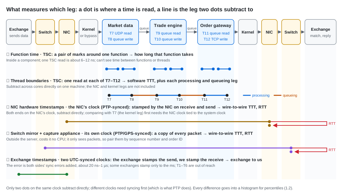
| Method | Clock | Where the time is read | Leg it measures | What it misses, what to watch |
|---|---|---|---|---|
| ① Function marks | TSC | Function entry, exit | One function by itself | Time between functions and threads |
| ② Thread-boundary marks | TSC | T7–T12 | Software TTT, each processing and queueing leg | The NIC and kernel legs |
| ③ NIC hardware timestamps | The clock on the NIC (PHC), usually PTP-synced | NIC receive, send | Wire-to-wire TTT, RTT | Comparing with T7 first needs the NIC clock tied to the system clock |
| ④ Switch mirror + capture appliance | The appliance’s own clock, usually PTP- or GPS-synced | Switch in, out | Wire-to-wire TTT, RTT | Sees only packets; pair them by sequence number and order ID |
| ⑤ Exchange timestamps | Two: the exchange’s clock stamps the send time, ours stamps the receive time, both synced to UTC | Exchange send, our receive | Exchange to us (one way) | The error is both sides’ sync errors added, about 20 ns–1 µs; some exchanges stamp only to the ms; inside the exchange is out of reach |
- Which to use: for tuning your own code, ① and ②; for reporting TTT externally, ③ or ④; when you suspect the network or the exchange got slower, RTT and ⑤.
- When two points subtract directly: when they are on the same clock. ① and ② are on this machine’s TSC, ③ on the NIC, ④ on the capture appliance; comparing across clocks needs syncing first, and the error is the sync error.
- PTP is not a sixth method: it is a clock-sync protocol (Precision Time Protocol). A master clock, usually fed by GPS, sends messages at intervals; each machine’s NIC hardware-timestamps them, works out from the round trip how far its own clock is off, and steers it back. It only makes different devices’ clocks tell the same time and measures no leg of the trading path itself. ③, ④ and ⑤ can be compared across devices because of it.
- Two things that don’t take times:
perftells you which function the time goes to (1.4), and the histogram turns the measured differences into percentiles (1.2, item 5).