
One memory access takes about 100 ns and brings back one 64-byte cache line. If only one request could be on the road at a time, one core would read memory at:
$$ \frac{64\ \text{B}}{100\ \text{ns}} = 0.64\ \text{GB/s} $$Yet the plainest loop, summing a multi-gigabyte array from start to end, runs at 15–60 GB/s on one core: 20 to 90 times that figure. No single access got faster; each still takes about 100 ns. Where does the extra speed come from?
Now walk a linked list over the same memory. Every step really does pay the full 100 ns, and you get exactly 0.64 GB/s. Same memory, same core, and the two loops are two orders of magnitude apart.
To explain it, separate two quantities: latency and bandwidth. “Memory is slow” can mean either one. This post sets up the two quantities first, then looks at what ties them together.
1. Two Quantities: Latency and Bandwidth
1.1 Latency and Bandwidth: The Road Between the Boxes
The earlier posts were about the boxes on the hardware map: L1D, L2, L3, the memory controller, the DIMMs (see the hardware map). Latency and bandwidth are about the road between the boxes:
- Latency: the time from the core issuing a load to the data landing in a register. The farther it goes, the longer it takes: an L1 hit stays inside the core, a memory access travels all the way to the DIMM and back.
- Bandwidth: how many bytes that road delivers per unit of time, in GB/s.
Think of a highway. Latency is how long one car takes to drive from A to B; bandwidth is how many cars arrive at B per hour. Adding lanes doesn’t make a single car faster; it only lets more cars be on the road at once.
1.2 Typical Numbers per Level: The Two Columns Fall at Different Rates
At about 4 GHz, as ranges for intuition:
| Level | Latency of one access | Bandwidth one core gets (sequential reads) |
|---|---|---|
| L1D | ~1 ns (4–5 cycles) | ~150–400 GB/s (2–3 loads per cycle, 32–64 B each) |
| L2 | ~3–5 ns | ~80–200 GB/s |
| L3 | ~10–30 ns | ~30–150 GB/s |
| Memory | ~70–120 ns | ~15–60 GB/s. The whole chip depends on the channel count: ~50–100 GB/s with 2 channels |
Both columns get worse level by level, but at different rates: from L1 to memory, latency grows about 100×, while one core’s bandwidth drops only about 10×. That alone shows they aren’t two ways of writing the same quantity.
One more premise: an “access” here is always one whole cache line, 64 B on x86. Even if you want 1 byte, 64 B travel down the road.
1.3 Little’s Law: Bandwidth ≠ 1/Latency
Back to the opening number. 0.64 GB/s is the bandwidth with one request on the road at a time. The real 15–60 GB/s is 20–90 times higher, and that factor is the number of requests in flight (outstanding requests). How many a core can keep in flight at once is its memory-level parallelism (MLP). Written as a formula, this is Little’s law from queueing theory:
$$ \begin{aligned} \underbrace{L}_{\text{requests in flight}} &= \underbrace{\lambda}_{\text{requests completed per second}} \times \underbrace{W}_{\text{latency}} \\ \text{bandwidth} = \lambda \times 64\ \text{B} &= \frac{\text{requests in flight} \times 64\ \text{B}}{\text{latency}} \end{aligned} $$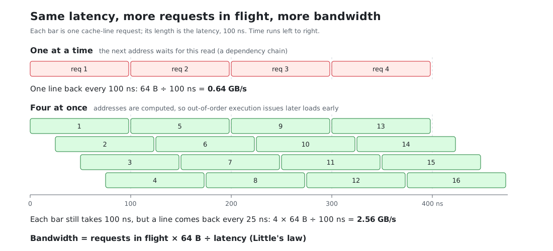
Run it backwards: one core reading 35 GB/s with 80 ns latency has
$$ 35\ \text{GB/s} \times 80\ \text{ns} = 2800\ \text{B} \approx 44\ \text{cache lines} $$on the road on average. High bandwidth doesn’t mean each request got faster. It means more lanes and more cars, and every car still drives the whole way.
1.3.1 Memory-Level Parallelism (MLP): What Keeps Requests in Flight
Three things:
- Out-of-order execution: a later load is issued without waiting for an earlier one to come back (#2 covered out-of-order execution and dependency chains). How far ahead it can look is set by the ROB; see 1.3.2.
- The LFB (line fill buffer; AMD calls it the MAB, papers call it an MSHR): a small table where L1D tracks which misses haven’t come back yet, 12–24 entries per core. That’s the most misses the core itself can have outstanding.
- Hardware prefetchers: once they see you walking sequentially, they send requests ahead on their own, without using your instructions. The L2 prefetcher parks its requests in L2’s own queue of outstanding requests (the L2 MSHRs, 30–60 entries), so it can keep another batch in flight beyond the LFB.
The 44 lines worked out above are more than the LFB’s 12–24 entries; the extra ones are the L2 prefetcher’s, held on your behalf. A core’s requests in flight fall into roughly three tiers:
| Access pattern | Requests in flight | One core’s bandwidth (at 80 ns) |
|---|---|---|
| The next address waits for this read (linked list) | 1 | 64 B ÷ 80 ns ≈ 0.8 GB/s |
| Independent addresses the prefetcher can’t help with (random, or a stride that crosses a page every time) | The LFB’s 12–24 entries | ~10–20 GB/s |
| Sequential reads, prefetchers at full speed | ~30–70 | ~15–60 GB/s |
1.3.2 The ROB and the Instruction Window: How Far Out-of-Order Execution Looks Ahead
The ROB (reorder buffer) is the ledger of out-of-order execution. On the hardware map it sits in the core’s top box (fetch → decode → out-of-order execute → retire) and handles the “out-of-order execute → retire” part. It isn’t on the road the data takes: it holds instructions that haven’t retired yet, not data. But how many memory accesses a core can put on the road at once depends on it.
x = a[i];      // (1) misses, goes to memory, ~80 ns
y = b[j];      // (2) independent of (1), also misses
s += x;        // (3) waits for (1)
t = y * 2;     // (4) waits for (2)
- In: in program order. Decoded instructions join the tail of the ROB one by one, one entry each (strictly, one micro-op each).
- Execute: whichever has its inputs ready goes first. (2) doesn’t wait for (1); as soon as its address is computed it’s issued, so the two misses are on the road together. (3) waits for the value of (1), (4) for the value of (2).
- Retire: only from the head, in order. Retiring makes a result official and frees the entry. Even if (2) comes back first, it waits until (1) has retired.
Why must retirement be in order? Unretired results are still drafts. When a branch was mispredicted or an exception fires, the core throws away every draft after the head, and the program still looks as if it ran one instruction at a time, in order.
The trouble is that one memory miss is long: 300–500 cycles. A missing load at the head of the ROB can’t retire, so everything behind it queues up, while the front end keeps adding 4–8 instructions per cycle at the tail. A 200–600-entry ROB fills in about 100 cycles (20–30 ns). Once it’s full, no new instruction gets in, and the core just waits out the remaining 50–100 ns. So the only loads that can overlap with this miss are the independent ones among the next 200–600 instructions. That stretch is the instruction window. With a 500-entry ROB:
| Code | Instructions between two independent misses | How many fit in the window | Which limit hits first |
|---|---|---|---|
Linked list p = p->next | The next address waits for this read | 1 | The dependency chain; a bigger ROB doesn’t help |
s += a[idx[i]], a large, idx shuffled | ~5 | ~100 | The LFB (12–24 entries) |
| A ~150-instruction hash before each table lookup | ~150 | ~3 | The ROB |
Put together (counting only the loads the core issues itself, not the prefetchers’):
$$ \text{misses in flight} \;\approx\; \min\Bigg(\underbrace{\frac{\text{ROB entries}}{\text{instructions between two independent misses}}}_{\substack{\text{how many the window holds} \\ \text{(just 1 for a dependency chain)}}},\;\; \underbrace{\text{LFB entries}}_{\text{most it can track}}\Bigg) $$Strictly, the window is whichever of the ROB, the load queue and the physical registers fills first; the ROB is only the nominal limit. The load queue has just 70–200 entries, so in a loop dense with loads it fills before the ROB. Hardware prefetchers aren’t bound by this formula: their requests come from L1 and L2 themselves and take no ROB or load-queue entries, which is how sequential reads reach 30–70 in flight.
1.3.3 Channels, Ranks, Banks: Lanes, a Shared Lane, Loading Windows
Down at the DIMMs, this stretch of road has its own parallelism. The DRAM structure was covered in #6, section 3.4; here the only question is which quantity each level affects:
- Channels mainly set bandwidth. Each channel is an independent set of data lines that transfers on its own. The channel count is the lane count: dual channel roughly doubles total bandwidth over single channel, while the latency of one access barely changes.
- Ranks add no bandwidth. The ranks on one channel share its data lines, only one can transfer at a time, and switching ranks costs a few idle cycles. What they do is let one channel carry more banks.
- Banks affect both. On the bandwidth side, different banks can each open a row and prepare data independently, so the DRAM works on several requests at once: this is the DIMM’s share of the “requests in flight”. On the latency side, each bank’s row buffer decides how fast one access is: about 15 ns on a hit to the open row, about 40 ns when the old row must be closed and a new one opened first.
Channels decide how many lanes there are, banks decide how many windows in the warehouse can load goods at once, and the row buffer decides how long one window takes to load one car.
1.4 The Dependency Chain: Does the Next Address Wait for This Load?
To tell whether code is latency-bound or bandwidth-bound, ask one question: is the next load’s address known only after the previous load comes back?
1.4.1 Computed Addresses: Bandwidth-Bound
long long s = 0;
for (int i = 0; i < n; ++i)
    s += a[i];          // address i+1 is computed: &a[0] + 4(i+1); no need to wait for a[i]
The CPU can issue load after load and keep a pile of misses on the road. The bottleneck is how many can be in flight and how many bytes per second come back: bandwidth.
The column-walk experiment in #6, section 3.2, is this case. The index m[i * row_ints + j] is computed too, independent of the values read. So the 0.81 ns per access measured there is throughput (total time ÷ number of accesses), not the latency of one L2 access (about 5 ns). 5 ÷ 0.81 ≈ 6: on average six or seven misses are on the road at once. That is Little’s law.
1.4.2 Addresses That Come Back From Memory (Pointer Chasing): Latency-Bound
struct Node { int value; Node* next; };
for (Node* p = head; p != nullptr; p = p->next)   // next address = the p->next just read
    s += p->value;
Until p->next comes back, the next load doesn’t even have an address and can’t be issued. There’s only ever one car on the road, and every step pays a full latency. This is pointer chasing, the dependency chain from the denormalization section of #6. With the nodes out of cache, each step costs about 100 ns and you use only 0.64 GB/s: a wide road with a single car on it.
Common latency-bound structures: linked lists, std::map (a red-black tree, one pointer per level), hash-table collision chains, multi-level lookups (instrument, then account, then risk parameters).
1.4.3 Measuring Bandwidth vs Measuring Latency: One or Two Orders of Magnitude Apart
- To measure bandwidth: scan a large array sequentially, let prefetching and out-of-order execution run flat out, and compute GB/s.
- To measure latency: turn the array into a random cyclic permutation and do
k = q[k]each step, so the next address depends on the value just read. The prefetcher can’t guess it and out-of-order execution can’t help; compute ns per step.
On the same memory, the two methods can differ by one or two orders of magnitude. When someone quotes a memory number, first ask: which method was it?
1.5 Bandwidth Demand and Arithmetic Intensity: How Fast the CPU Wants Data
Everything above is the supply side: how many bytes per second each level can deliver. Whether bandwidth is the bottleneck also depends on the demand side: if data arrived for free, how many bytes per second would the loop consume? That’s its bandwidth demand. It’s set by the arithmetic intensity, the number of operations per byte moved: the less work per byte, the faster the loop eats. Take the smaller of the two:
$$ \text{actual speed} \;=\; \min\big(\,\text{bandwidth demand},\;\; \text{what the level holding the data can deliver}\,\big) $$That is the heart of the roofline model. One core at about 4 GHz:
| Loop | Bandwidth demand | Bandwidth-bound from which level |
|---|---|---|
int sum s += a[i], not vectorized, one accumulator, one add per cycle | 4 B/cycle × 4 GHz = 16 GB/s | Only memory barely keeps up. In L1/L2/L3 the bottleneck is the add chain, not bandwidth |
| SIMD-vectorized, several accumulators (AVX2, two 32 B loads per cycle) | 64 B/cycle × 4 GHz = 256 GB/s | As soon as data leaves L1: L2’s 80–200 GB/s can’t keep up |
| 100+ operations per element | Under 1 B per cycle | Almost always compute-bound, even with the data in memory |
The less work per byte and the more vectorized the loop, the sooner it hits bandwidth. The same sum runs 16× faster once vectorized, but it’s stopped by bandwidth the moment data leaves L1. The scalar version is slow on its own; bandwidth only catches up with it at the bottom level. This is also why a “bigger array, slower loop” curve comes in steps: every time the array falls out of a cache level, the supply side drops to the next tier, and whenever that tier is below the demand, the speed drops a step with it.
The measurement in #6 fits: the row walk reads one 4 B int in about 0.05 ns, and 4 B ÷ 0.05 ns = 80 GB/s (with the matrix in L2). A scalar loop can’t go that fast, so the compiler vectorized it. It levels off around 80 GB/s, right inside the range one core gets from L2 (80–200 GB/s).
The HFT hot path is the opposite: each market-data message touches a few cache lines, the bandwidth demand is tiny, and bandwidth is almost never the bottleneck. What hurts is the latency of 1.4.2. Bandwidth is the bottleneck in batch work: market-data replay, backtests, log flushing, big copies.
1.5.1 Vectorization (SIMD) and Multiple Accumulators: Who Does It
- Vectorization (also SIMD, single instruction multiple data): one instruction works on a whole row of values. An AVX2 vector register is 256 bits (32 B) wide and holds 8
ints or 8floats, so one add instruction does 8 additions where a scalar loop does 1. One vector load reads 32 B and fills exactly one register, and most cores can issue 2 loads per cycle: that is the table’s “two 32 B loads per cycle”. You can leave it to the compiler (-O3, plus-mavx2or-march=nativeto allow AVX2; by default it uses only 16 B-wide SSE) or write intrinsics by hand (compiler built-in functions such as_mm256_add_epi32). - Multiple accumulators: in
s += a[i]each step waits for the previous result, and that chain is the dependency chain. With one accumulator the adds run one after another and the load ports can’t be kept fed. Splittingsinto several independent accumulators and combining them at the end lets several adds run in the execution units at the same time, which is instruction-level parallelism (ILP). How many you need is Little’s law again: $\text{adds in flight} = \text{adds completed per cycle} \times \text{add latency}$. Vector integer adds have a latency of about 1 cycle, so 2 × 1 = 2 accumulators are enough.floatadds take 3–4 cycles, so you need 2 × 3–4 = 6–8.
Whether the compiler does it for you, as GCC actually behaves:
| Sum | Vectorized | Split into several accumulators |
|---|---|---|
int | Yes, on its own (with -O3) | No, one accumulator |
float, no -ffast-math | No: floating-point addition isn’t associative, and a different order changes the last few bits | No: scalar adds, one chain |
float, with -ffast-math | Yes, on its own | No, one accumulator |
So the compiler vectorizes an int sum by itself, and a float sum only with -ffast-math. It splits accumulators in neither case (-funroll-loops just writes the same dependency chain out several times); you write that by hand. Whether one accumulator is enough depends on where the data is and how long an add takes:
- An
intadd takes 1 cycle: one 32 B load per cycle, about 128 GB/s. Enough with the data in L3 or memory (15–150 GB/s); too slow with it in L1/L2 (80–400 GB/s). - A
floatadd takes 3–4 cycles: one 32 B load every 3–4 cycles, about 32–43 GB/s. Barely enough with the data in memory (15–60 GB/s); it can’t keep up with L1, L2 or L3.
Other compilers (clang, for example) behave differently; check the assembly.
1.6 The Big Picture: Total Time = Lines to Move × Time per Line
Without “how much to move” and “how fast it moves” in one formula, discussions go in circles: one moment the bottleneck is bandwidth, the next it “degrades into serial and exposes latency”. Put together:
$$ \text{total time} \;\approx\; \underbrace{\text{lines to move}}_{\substack{\text{Q1 bytes used per line} \\ \text{Q2 does the line survive until reuse}}} \;\times\; \underbrace{\text{time per line}}_{\substack{\text{Q3 which level it comes from} \\ \text{Q4 how many are in flight}}} $$Inverted, the time per line is the number of lines moved per second. It has two ceilings, and the lower one wins:
$$ \text{lines per second} \;=\; \min\Bigg(\underbrace{\frac{\text{requests in flight}}{\text{latency}}}_{\substack{\text{one core hits this first} \\ \text{(Little's law)}}},\;\; \underbrace{\frac{\text{peak bandwidth}}{64\ \text{B}}}_{\substack{\text{usually only hit with} \\ \text{many cores pushing}}}\Bigg) $$Finally, take the minimum with the bandwidth demand from 1.5:
$$ \text{actual speed} \;=\; \min\big(\,\text{bandwidth demand},\;\; \text{useful bytes per line} \times \text{lines per second}\,\big) $$1.6.1 Four Questions: Locality, Hit Level, MLP
- Q1 How many bytes of each line are used (spatial locality). Reading
ints contiguously, one 64 B line feeds 16 of them. With a stride of 64 B or more, each line yields 4 B, so the same useful data needs 16× the lines. That’s what “wasting bandwidth” means, and it has nothing to do with whether the bus is busy. A 64 B stride already makes this question as bad as it gets; a larger stride is no worse. - Q2 Does a line survive until it’s used again (temporal locality). There are only three reasons it doesn’t: compulsory misses (first touch, unavoidable), capacity misses (more lines to reuse than the level holds), and conflict misses (addresses crowding into one set, the critical stride of #6, section 3.1). Padding only cures conflicts.
- Q3 Which level does it come from. This sets latency and peak bandwidth: the table in 1.2.
- Q4 How many can be in flight. If the next address waits for this read (1.4.2), there’s just 1, and every line pays a full latency. If addresses are computed (1.4.1), out-of-order execution issues later loads early, each miss takes an LFB entry, up to N of them (12–24), and each line costs $\text{latency} / N$. Prefetchers can add another batch on top. This is what “pipelining hides latency” means: latency doesn’t get shorter; many waits overlap. How far ahead the core can look is limited by the ROB, how many it can track by the LFB, and a dependency chain can’t be pulled forward at all.
When you read any claim about memory access, first ask which question it answers. If one paragraph mixes several, take them apart.
1.6.2 Three Easy Confusions
- A full LFB doesn’t mean “degraded to serial”. Full is exactly when overlap is greatest: all N entries are on the road, miss N+1 waits for the oldest to return and free its slot, and in steady state N are always in flight, so each line costs $\text{latency} / N$ (80 ns and 16 entries: one line every 5 ns). Only a dependency chain is truly serial. So bandwidth and latency aren’t either-or: one core’s bandwidth is itself $\text{requests in flight} \times 64\ \text{B} / \text{latency}$, and when latency grows (DRAM row conflicts, TLB misses), the same N moves fewer lines per second.
- “Bandwidth-bound” has two ceilings. One core usually hits $\text{requests in flight} / \text{latency}$ first (one core reads memory at about 15–60 GB/s); the chip’s bus peak is usually reached only with many cores pushing (2 channels already give 50–100 GB/s). Even then, reads reach only 70–90% of the peak: refresh, read/write turnarounds and bank conflicts all take time. Also, “5 ns per line” is the inverse of throughput, not latency; every line still takes the full 80 ns. Calling it an “effective latency” is exactly where the confusion comes from.
- Padding cures conflicts, not capacity. The
int m[64][1040]in #6 has only 64 rows; a column walk touches 64 lines, which all fit in L1D (512 slots) once spread across the sets, so columns 1–15 all hit in L1. With 2048 rows, one column is 2048 lines (128 KiB): padding spreads them evenly over the 64 sets, but that’s 32 lines fighting for 8 ways in each set. After column 0, L1D holds only the last ~512 rows, so column 1 misses in L1 from row 0 on and hits in L2. To hit in L1 you also need tiling: walk only a stretch of rows that fits in L1, finish all 16 columns for that stretch, then move to the next.
1.7 Loaded Latency: Bandwidth Fills Up, Latency Rises
The more cars on the road, the closer it gets to the lanes’ limit, and queues start forming. The memory controller is no different: the fuller the chip’s bandwidth, the higher the latency of each access. Near the limit it can exceed 2× the idle latency. This is loaded latency.
What it means for HFT:
- The hot path is “receive a market-data message → look up the order book → decide → send an order”: a chain of dependent accesses on a tiny amount of data. What hurts is latency.
- But the memory controller and L3 are shared by all cores. When another process on the same chip is scanning memory hard (a backtest, log flushing, market-data replay), bandwidth fills up and every miss on the hot path has to queue. Pinning and isolating cores isolates the compute, not this road (#1).
- So on production machines, either move such bandwidth-hungry jobs elsewhere or limit them with the hardware’s allocation features: Intel CAT partitions L3, and MBA throttles each core’s memory bandwidth.
2. The Bandwidth Side: Capacity, Writes, Many Cores
Zero a 1 GiB block of memory with the plainest loop:
void plain_zero(int* dst, size_t n) {
    for (size_t i = 0; i < n; ++i) dst[i] = 0;
}
There is not a single load in the code, yet 2 GiB cross the memory bus, and half of it is reads. On the same core, a 16 KiB array is read at hundreds of GB/s and a 256 MiB array at a few tens. And on a 64-core chip with a ~300 GB/s peak, one core scanning memory alone gets a small slice of it. All three answer the two quantities in Part 1’s overall picture: how many lines must move, and how wide the road is.
2.1 Working Set: Which Level the Data Fits In
The working set is the bytes a piece of code keeps touching over a stretch of time. Whichever level the working set fits in is where the repeated accesses hit, and that level’s speed is the speed you get.
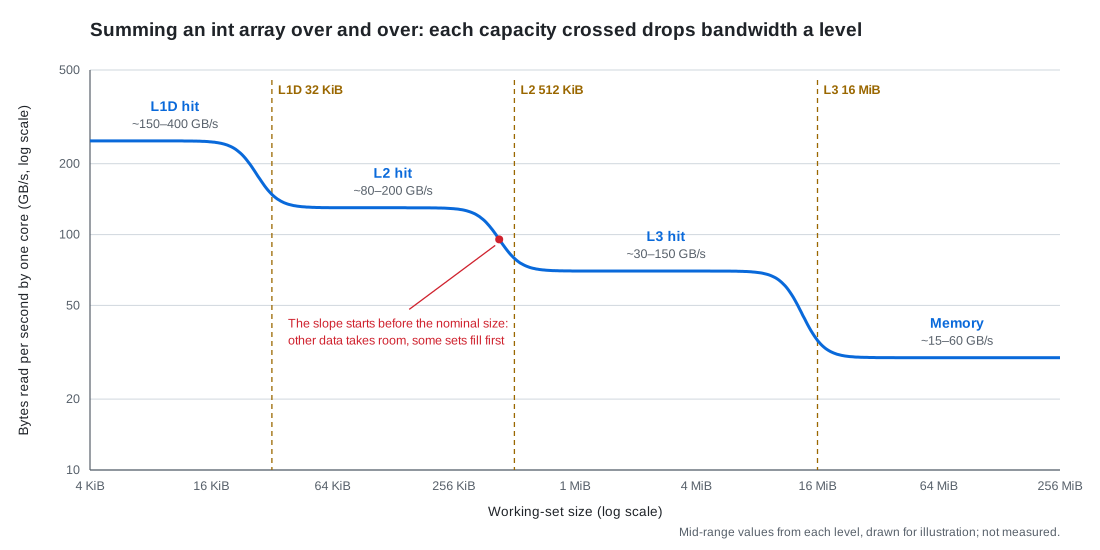
Sum an int array sequentially, over and over, growing the array from 16 KiB to 256 MiB, and measure the bytes read per second at each size:
// a holds n ints; n × 4 B is the working set; scan it reps times
for (int rep = 0; rep < reps; ++rep)
    for (size_t i = 0; i < n; ++i) s += a[i];
On a machine with a 32 KiB L1D, 512 KiB L2 and 16 MiB L3, the curve has four steps (estimated from the ranges on the quick reference):
| Working set | Hits in | One core, sequential read |
|---|---|---|
| ≤ ~32 KiB | L1D | ~150–400 GB/s |
| ~32 KiB – 512 KiB | L2 | ~80–200 GB/s |
| ~512 KiB – 16 MiB | L3 | ~30–150 GB/s |
| > ~16 MiB | Memory | ~15–60 GB/s |
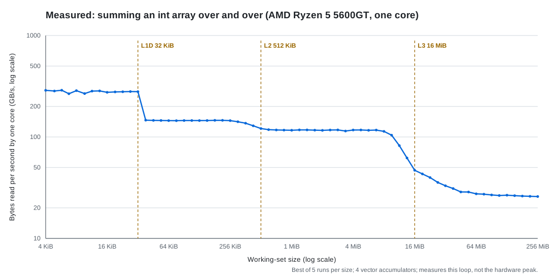
One measured run (Ryzen 5 5600GT, one core, GCC 16.2.0,
-O3 -march=native, four vector accumulators, best of 5 runs per size; this measures the loop itself, not the hardware peak):
- All four plateaus land inside the ranges the schematic gives: L1D ~280 GB/s (267–289), L2 ~145 (144–146), L3 ~116 (114–117), memory ~26 (25.9–27.5).
- Knees versus the dashed lines: L1D→L2 cuts right at the 32 KiB line (32 KiB still reads 279 GB/s; the next point, 39 KiB, is already down to 146). The L2→L3 slope starts around 300 KiB — before the 512 KiB line — and is already most of the way down at the line (121 GB/s), settling onto the L3 plateau by 1 MiB. The L3→memory slope starts around 9 MiB, slightly before the 16 MiB line, where it is only halfway down (~47 GB/s); the victim cache does not push the knee right as a whole — what runs late is the end of the slope: 32 MiB still reads ~33 GB/s, and only around 48 MiB does it settle onto the memory plateau of 26 GB/s. Leaving L3 behind is gradual.
- Why the L3 tail runs out to ~48 MiB: if L3 replaced lines in strict LRU order, a sequential scan of an array larger than L3 would evict every line before its reuse, the hit rate would drop straight to 0, and the curve would fall off a cliff near 16 MiB. The measured curve falls gradually, which says L3 replacement is not pure LRU: each pass, some lines happen to survive. The larger the array, the smaller the surviving share, roughly $\text{L3 size} / \text{working set}$: about half at 16 MiB, and only around 48 MiB does it reach the memory plateau.
Past each capacity, the lines you keep reusing go from “fits in this level” to capacity misses that come from the next level down. Four things to watch when reading the curve:
- The knee comes early, and it is a slope, not a corner. Other data takes room too: the stack, code, page-table entries. Set associativity is not perfect LRU either: L2 and L3 pick the set by physical address, the OS hands out scattered physical pages, and some sets fill and start evicting before the whole cache is full. L3 is also shared by every core.
- On some chips the knee comes late. When L3 is a victim cache of L2 (lines enter L3 only when L2 evicts them, and L3 keeps no second copy of what L2 holds), the total capacity is about L2 + L3.
- Sequential steps are shallower than random ones. This chart measures each level’s bandwidth; that is what the experiment is for, not a shortcoming of it. With sequential reads, prefetchers fetch ahead and many requests are in flight, so most of the next level’s latency is hidden and bytes per second are set by each level’s bandwidth: about 10× from L1 to memory. To see latency you need a different experiment: random pointer chasing, where the next address waits for this load, no prefetching, one at a time, and each step pays a full latency: about 100× from L1 to memory. The two curves answer two different questions.
- Random access adds one more step for the TLB: once the working set exceeds the few MiB the TLB covers, every access pays an extra page walk.
The hot path’s data structures (order book, positions, parameter tables) have to fit in L1/L2 before “a few nanoseconds per access” is on the table. The compact layouts from #6 save more than lines: they move the working set up a level.
2.2 Write Misses and RFO: One Line Written, Two Trips on the Bus
A store goes into the store buffer first. Before it can be written into L1D, the core needs exclusive ownership of the line (the I→M step in MESI). If the line isn’t in the cache, the whole line must first be read from memory and then modified. This is RFO (read for ownership). The reason is that caches manage whole 64 B lines: you wrote 4 B, and the other 60 B still have to be correct. Allocating the line into the cache on a write miss is called write-allocate.
The modified line is dirty, and when it is evicted it is written back to memory (write-back). So an ordinary store moves each line across the bus twice:
$$ \text{bus traffic} \;=\; \underbrace{64\ \text{B}}_{\text{RFO read}} \;+\; \underbrace{64\ \text{B}}_{\text{write-back on eviction}} $$- Zeroing 1 GiB (far larger than L3), as in the opening example, moves 2 GiB over the bus. Write bandwidth computed as “bytes written ÷ time” is only half the bus traffic.
memcpyof 1 GiB: read 1 GiB of source, RFO 1 GiB of destination, write back 1 GiB, 3 GiB in total, of which 2 GiB is useful.
The store buffer hides only the latency of a store: later instructions don’t wait for it. It has 50–110 entries, and a store-dense loop fills it; then the core stalls, and RFO bandwidth sets the speed.
How much is RFO bandwidth? It depends on where the line is:
$$ \text{one core's useful write bandwidth to memory} \;\approx\; \frac{\text{RFOs in flight} \times 64\ \text{B}}{\text{latency}}, \qquad \text{chip's useful write bandwidth} \;\lesssim\; \frac{\text{chip peak} \times (70\%\text{–}90\%)}{2} $$- The line is already in L1/L2 and owned by this core: no RFO; the store ports set the speed. 1–2 stores of 32 B per cycle at 4 GHz is about 130–250 GB/s. A hot path rewriting the same few lines is in this case.
- One core writing an array far larger than L3: bound by how many RFOs are in flight. RFOs occupy LFB entries like read misses, and the L2 prefetcher issues RFOs ahead for sequential stores too, so the arithmetic is the same as for reads: about 10–40 GB/s of useful write bandwidth, usually somewhat below the same core’s sequential read, because write-backs also use the road and the store buffer hands stores over in order.
- Many cores writing together: they hit the chip’s bus. Every line written crosses it twice (RFO + write-back), so useful write bandwidth is at most about half the peak, and with read/write turnaround only 35%–45% of it. On a 2-channel chip with a 50–100 GB/s peak, all cores writing get about 20–40 GB/s of useful writes.
These are worked out from the read-side numbers. NT stores turn the two bus trips into one, and the chip’s useful write bandwidth climbs back to 70%–90% of peak.
Reads and writes are asymmetric in one more way: the DRAM data bus is shared by both directions, and switching from reads to writes and back costs idle cycles, so a mixed read/write stream reaches a lower fraction of peak than pure reads. Some CPUs optimize bulk string instructions like rep stosb / rep movsb: knowing the whole line will be overwritten, they skip the RFO. glibc’s large memset / memcpy use them, or the streaming stores in the next section.
2.3 Non-Temporal Stores: No Read-Back, No Cache
A non-temporal store (NT store; non-temporal means “not reused soon”) is a different store instruction (movnti, movntdq on x86; intrinsics such as _mm_stream_si128). It neither reads the line back nor puts it in the cache: stores to the same line are collected in a write-combining buffer (WC buffer; on Intel it shares the 12–24 LFB entries), and once 64 B are complete the whole line is written straight to memory. One trip on the bus, so memcpy goes from 3 trips to 2.
#include <immintrin.h>
// dst aligned to 16 B, bytes a multiple of 64 (whole lines written)
void stream_zero(void* dst, size_t bytes) {
    __m128i z = _mm_setzero_si128();
    auto* p = static_cast<__m128i*>(dst);
    for (size_t i = 0; i < bytes / 16; ++i) _mm_stream_si128(p + i, z);
    _mm_sfence();   // NT stores are weakly ordered: sfence before publishing "done"
}
Three traps:
- Write whole lines, contiguously. Write half a line and the WC buffer is flushed early as several partial writes, slower than ordinary stores.
- They are weakly ordered. Ordinary x86 stores become visible in order (TSO, #2); NT stores are the exception. Writing a batch of data and then a “ready” flag needs
_mm_sfence()in between, or another core may see the flag before the data. - The data lands in memory, not in cache. Any cached copy of the line is invalidated too. Whoever reads it next, you or another core, pays a full memory miss, about 80–120 ns.
So it suits data that is written in bulk and not read soon: copies larger than L3, log writes into a big file buffer. glibc’s memcpy switches to NT stores above a threshold on the order of the L3 size. The opposite case is an inter-core SPSC queue (#4, #5): what goes in is read by another core right away, and NT stores would push the data out to memory only for the consumer to pull it back.
2.4 Shared Bandwidth Across Cores: Which Ceiling Belongs to Whom
L3, the memory controller and the channels are shared by all cores. The two ceilings from Part 1’s overall picture split cleanly once more cores join:
$$ \text{one core alone} \;\approx\; \frac{\text{requests in flight} \times 64\ \text{B}}{\text{latency}}, \qquad \text{each of k cores together} \;\approx\; \min\Big(\text{alone},\;\; \frac{\text{chip peak} \times (70\%\text{–}90\%)}{k}\Big) $$- One core alone hits the first ceiling. 40 in flight at 100 ns: 40 × 64 B ÷ 100 ns ≈ 25.6 GB/s, regardless of how many channels the chip has.
- Many cores hit the second. On a 2-channel chip with a ~50–100 GB/s peak, 2–4 cores scanning together saturate it. Add more cores and the total stays flat, each core’s share shrinks, and latency climbs (loaded latency, section 1.7).
- Chips with many channels are chips with many cores. 8–12 channels and ~200–500 GB/s come with 32–128 cores; with every core scanning, each gets a few GB/s, less than one core alone. The on-chip path on such chips is longer and memory latency is often higher, so one core alone also takes only a small fraction of the peak.
- More channels raise only the second ceiling. For one core alone, extra channels barely help. Raising the first ceiling takes more requests in flight (prefetching, removing dependency chains) or shorter latency. Locking the core frequency high (#1) doesn’t raise it either: the DRAM part of the trip doesn’t shrink in nanoseconds with core frequency, and a faster core just counts more cycles per miss.
The hot path uses very little bandwidth; what it cares about is queuing once someone else saturates the second ceiling. Bandwidth-hungry jobs such as backtests, market-data replay and logging belong on another machine or another NUMA node, or under an MBA limit.
3. The Latency Side: The Bill for One Miss, TLBs, Prefetching, NUMA
The same hash-table lookup takes about 90 ns on one machine; move it to a dual-socket server where another thread initialized the memory and it takes about 180 ns; move the table from 4 KiB pages to 2 MiB pages and it drops by another 20 ns or so. Not a line of code changed. What changed is how far this one load has to travel. This part breaks the latency of one miss into segments, then looks at what TLBs, prefetching and NUMA each add to the bill or hide from it.
3.1 One Miss, Itemized: Where 80–120 ns Goes
On the quick reference’s hardware map this is the four-step load path: translate the address, look up each cache level, have the memory controller fetch from the DIMM, and bring the whole line back the same way. Split one load that goes all the way to memory into segments (the split is for intuition; chips differ a lot):
$$ \text{latency of one load} \;\approx\; \underbrace{t_{\text{TLB}}}_{\substack{\text{hit: 0} \\ \text{miss: 15–30 ns}}} + \underbrace{t_{\text{L1}} + t_{\text{L2}} + t_{\text{L3}}}_{\substack{\text{check each level, all miss} \\ \text{~15–35 ns}}} + \underbrace{t_{\text{to controller}}}_{\substack{\text{on-chip network} \\ \text{~10–30 ns}}} + \underbrace{t_{\text{DRAM}}}_{\substack{\text{row hit / empty / conflict} \\ \text{~15 / 30 / 40 ns}}} + \underbrace{t_{\text{return}}}_{\substack{\text{back, filling each level} \\ \text{~10–20 ns}}} $$With a TLB hit, that adds up to about 80–120 ns. Three points:
- DRAM itself is only about a third. A DIMM’s CAS latency converted to nanoseconds has stayed around 13–16 ns from DDR3 to DDR5; each generation raised bandwidth, not latency. Faster DIMMs barely change the latency of one miss.
- More cache levels and bigger chips make “not found” itself more expensive. Each level has to finish its lookup and report a miss before the next is asked, and the bigger the L3 slices and the on-chip network, the longer the trip. Chips with many cores often have longer memory latency, which is why one core alone gets so little of the peak (2.4).
- On top of the 80–120 ns come four kinds of extra wait: a TLB miss (3.2), an address on the other socket (3.4), a DRAM refresh (up to ~300–500 ns more in the worst case, #6), and a bus saturated by others (loaded latency, 1.7, 2× or more). A hot path’s P99 is mostly these stacking up.
3.2 TLB and Huge Pages: The Translation Step
This is step 1 of the load path. First the prerequisite: programs use virtual addresses, the DIMMs understand physical addresses. The OS manages the mapping in pages (4 KiB by default): the low 12 bits of a virtual address are the offset within the page and don’t change in translation; the high bits are the page number, which has to be looked up in the page table to find its physical page. x86-64 page tables have 4 levels, so one lookup reads 4 page-table entries in turn. Doing that on every load would be far too slow, so the CPU caches recent translations in the TLB (translation lookaside buffer).
The TLB has two levels too, each entry covering one page:
| TLB | Entries | Covers with 4 KiB pages |
|---|---|---|
| L1 dTLB | 64–96 | ~256–384 KiB |
| L2 TLB (STLB) | 1500–3000 | ~6–12 MiB |
When the working set exceeds the STLB’s reach and the access pattern is random, almost every access has to walk the page table: a page walk. Random reads over a 1 GiB array, for example: 1 GiB ÷ 4 KiB = 262,144 pages, against 1500–3000 STLB entries, a hit chance of about 1%.
A page walk costs only about 15–30 ns extra, not four more memory accesses, for two reasons: page-table entries are ordinary data, and the frequently used lines sit in L1/L2/L3; and the CPU has page-walk caches holding the upper levels, so usually only the last level is read. When the page-table entries themselves miss in cache (huge, very random working sets), one walk costs a memory access or more, and the latency can double.
Huge pages attack both ends:
- One entry covers 2 MiB, 512× the reach. The same STLB covers several GiB; a 1 GiB array needs only 512 entries, which fit, and page walks all but disappear.
- One fewer page-table level: a 2 MiB translation stops at level 3, so the walk itself is shorter.
This is also the extra TLB step mentioned in 2.1: the latency curve for random access drops one more level once the working set passes a few MiB. Putting the hot path’s large tables (order book, id maps) on huge pages removes that level.
3.3 Hardware and Software Prefetching: Hiding Latency, Within One Page
A hardware prefetcher watches your access pattern and issues requests for lines you’ll need later, without costing you instructions. It doesn’t make a miss shorter; it starts the miss before you need the data, so more requests are in flight (1.3: sequential reads reach 30–70 in flight because of it). Two common kinds:
- L1 prefetchers: the next line (next-line), or a fixed stride per load instruction (IP-stride).
- The L2 streamer: recognizes an ascending or descending stream and runs 10–30 lines ahead; its requests sit in L2’s MSHRs, not in the LFB.
It usually doesn’t cross a 4 KiB page. Caches from L2 down work on physical addresses, and that’s all the prefetcher has. The next page in virtual address order could be anywhere physically; finding out takes a translation, and the L2 prefetcher has no TLB to ask. So a stream stops at the page boundary, the next page has to be recognized afresh, and its first few accesses are ordinary misses. With a large stride (say 8 KiB per step), every step crosses a page and the prefetcher can’t help at all; that is one reason walking a big matrix by column is slow in #6. (Some newer chips can cross 4 KiB boundaries inside a 2 MiB huge page; it depends on the implementation.)
Two kinds of access a prefetcher can’t guess: pointer chasing (the next address waits for this load, and nobody can issue it early) and random access (no pattern). For the second, if you know the addresses ahead of time, use a software prefetch:
// a batch of order ids, each looked up in a hash table; prefetch the slot D ids ahead
void lookup_batch(const uint64_t* ids, size_t n, const Slot* slots, uint64_t mask, size_t D) {
    for (size_t i = 0; i < n; ++i) {
        if (i + D < n) __builtin_prefetch(&slots[hash(ids[i + D]) & mask]);
        process(slots[hash(ids[i]) & mask]);
    }
}
How far ahead is Little’s law again: the prefetch has to go out one full latency early,
$$ D \;\approx\; \frac{\text{latency of one miss}}{\text{time to process one element}} $$- 100 ns latency and 5 ns per element: D ≈ 20.
- D too small: the data is still in flight when you need it, so you still wait, just less.
- D too large: too many prefetches in flight fill the LFB and block real misses; or the line arrives in L1 and waits so long that other data pushes it out, a wasted trip.
On a hot path the more common form is to gather such lookups into a batch: when one market-data message needs several tables, compute all the addresses first, prefetch them together, then use them in turn, so the misses overlap.
3.4 NUMA Remote Memory: One Machine, Two Distances to Memory
This is the socket and memory-controller layer of the hardware map. On a multi-socket server each socket has its own memory controller and DIMMs, forming a NUMA node. Reading local memory takes about 80–120 ns; reading the other socket’s memory goes over the inter-socket link first, about 120–200 ns, and the link’s bandwidth is lower than local memory’s.
Which node a physical page lands on is decided by default on first touch: the node of the thread that first writes the page. A common trap:
- An init thread on node 0
memsets the order book and market-data buffers, so every physical page lands on node 0. - The strategy thread is pinned to an isolated core on node 1, and every miss on the hot path is a remote access, 40–100 ns more for nothing.
- Pinning the thread doesn’t move the memory. Either have a thread pinned on the target node do the first write, or start with
numactl --cpunodebind=1 --membind=1(ormbind/ libnuma) to place the memory on node 1.
One more runtime trap: Linux’s automatic NUMA balancing (kernel.numa_balancing) periodically marks pages inaccessible, uses the resulting faults to see who touches them, and migrates them. For a hot path that means page faults and TLB shootdowns out of nowhere, so it is usually turned off on low-latency machines (#1).
In Practice
The multiple accumulators of 1.5.1 match the B1 Serial Accumulator card below: what perf shows, how to fix it, how to verify the fix.
- Signal: one
vaddss/vfmadddominates annotate (samples often land on the instruction after it, so look one back); IPC ≪ 1 while cache misses stay low. That combination is the key.- Cause: every
+=waits for the previous result, so the speed is set by the latency of a floating-point add (4–5 cycles) rather than its throughput (about 0.5 cycles), a gap of 8–10 times.- Fix: split into several independent accumulators. Four in plain C is about 4 times faster; SSE2 vector accumulation 4–8 times; AVX2 vectors with 4 accumulators 8–15 times.
- How many accumulators: $\text{latency} \div \text{throughput} = 4 \div 0.5 = 8$. Four is usually enough; tight loops use 8.
- The tail: the leftover elements that don’t fill a group need multiple accumulators too, or small inputs fall back to serial.
- Precondition: the operation must be associative (add, multiply, min, max). The result shifts by a rounding error; if it must match bit for bit, this fix is out.
- Verify: the output agrees within rounding error, and IPC at least doubles.
- Mechanism: #9 Loop Optimization 3.2; the accumulator-count formula is in #2 3.5; whether the compiler splits it for you is in Memory Latency and Bandwidth 1.5.1; measured in the perf special, 4.6.