
Add up the even numbers among a million random integers in 0–199, and repeat that 64 times. Run the same code again after sorting the array first, and it is about 7 times faster. Not one value changed and the sum is identical; the only difference is whether “is the next number even?” follows a pattern.
Then compile both with g++ -O2, and they run at the same speed again. Both facts start from the branch predictor in the CPU’s front end: why it has to guess, how it guesses, what a wrong guess costs, and how the compiler can remove the branch altogether.
1. The Branch Predictor: Why the CPU Guesses and What a Wrong Guess Costs
1.1 Where It Sits: The Front End
Most of the quick reference’s hardware map is the data side: loads and stores, caches, memory. Branch prediction lives on the other side, the front end, which fetches and decodes instructions and feeds them to the back end. In order:
- Fetch: read a chunk of bytes from L1I (the instruction cache) at “the address of the next instruction”.
- Decode: split them into micro-ops (µops).
- Rename and enter the ROB: into the out-of-order window (the ROB is covered in Memory Latency and Bandwidth, 1.3.2).
- Execute: only here is a branch’s condition actually computed and its direction known.
- Retire: confirmed in program order.
The branch predictor sits next to step 1: for every chunk fetched, it answers on the spot “is there a branch in here, and where does it go?”, and the fetch unit fetches the next chunk from wherever it says.
1.2 Why It Has to Guess: The Pipeline Is Longer Than the Gap Between Branches
Put two numbers side by side:
- From fetch to execute, an instruction travels about 15–20 cycles (the pipeline depth).
- In ordinary code, one instruction in 5–7 is a branch (about 15%–20% of instructions). The front end fetches 4–8 instructions per cycle, so it meets a branch almost every cycle.
If fetch stopped at every branch and waited for it to execute, each branch would waste 15–20 cycles and the CPU would spend most of its time idle. So the front end doesn’t wait: it keeps fetching and executing down the predicted path. This is speculative execution. Speculative results sit in the ROB and may retire only once the branch is confirmed to have been predicted right.
1.3 How It Guesses: Direction, Target, History
Here “branch” means any instruction that changes where the next instruction is fetched from: the conditional jumps an if compiles to, call, ret, and indirect jumps such as virtual calls. The predictor always guesses the address of the next instruction, never a data value (a function’s return value is data in a register and needs no guessing). A branch needs two guesses: taken or not (direction) and where to (target). What is hard differs by kind:
Target: the BTB (branch target buffer) records, by the branch instruction’s address, where it went last time; about 4000–12000 entries. One lookup at fetch tells whether this chunk holds a known branch and where it goes.
Function returns: a
retalways jumps; the hard part is where to. The same function called from different places has to return to different places:void log_it() { /* … */ } // ends in a single ret void on_trade() { log_it(); update(); } // this time the ret returns here and runs update() void on_quote() { log_it(); quote(); } // next time the same ret returns here and runs quote()This is the job of the RAS (return address stack, 16–32 entries): when fetch sees a
call, it pushes “where to come back to”; when it sees aret, it pops the top and fetches from there. It is still a guess: the push and the pop happen at fetch, while theretactually executes, reading the return address from the call stack in memory, 15–20 cycles later, and only then is the guess checked. As long as everycallis matched by aret, it is almost always right. It goes wrong in two cases: call depth beyond the RAS’s capacity (deep recursion), or calls and returns that don’t pair up, such as a thrown exception orlongjmpthat skips therets of the frames in between, leaving stale addresses in the RAS that make the next fewrets mispredict.Indirect branches (virtual functions, function pointers,
switchjump tables): one instruction can go to many targets; the indirect target predictor records the target by “this instruction + recent history”.Direction: the simplest scheme gives each branch a 2-bit saturating counter: +1 when taken, −1 when not, clamped to 0–3, and predict “taken” at ≥ 2. It predicts loops well (taken 99 times, not taken once at the end, only the last one is wrong), and one odd outcome doesn’t flip its mind at once.
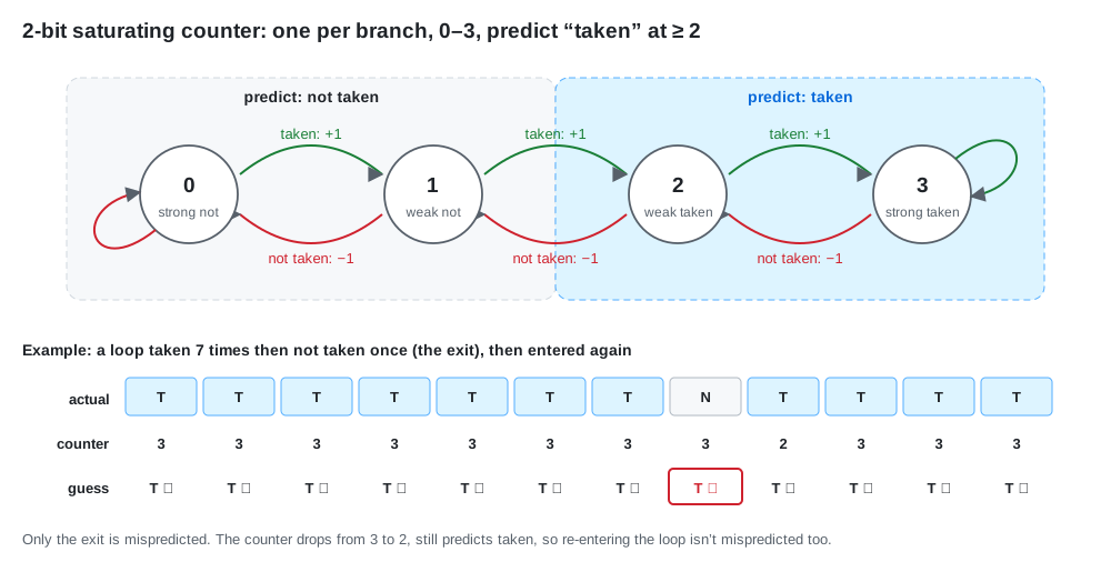
Modern predictors add history on top: the outcomes (taken / not taken) of the last 50–1000 branches, recorded as one global history string, are used together with the branch address to look up a table. That lets them learn patterns like “if the previous branch was taken, this one isn’t” or “taken once every 3 times”. The mainstream design (the TAGE family) uses several tables with different history lengths and picks the longest one that hits. The upshot: a branch with a pattern can be learned, even a long pattern; a branch without one can’t be learned by anyone. A condition that is a fresh 50/50 coin flip every time is predicted right half the time by even the best predictor.
In ordinary programs these structures together predict well over 95%–99% of branches.
1.4 What a Wrong Guess Costs: Flushing the Pipeline
When a branch executes and turns out to be mispredicted:
- Every instruction fetched after it (still in the pipeline, already in the ROB, even already executed) is discarded.
- Fetch goes back to the correct address and starts over.
- The new instructions go through fetch, decode and rename again before the back end fills up.
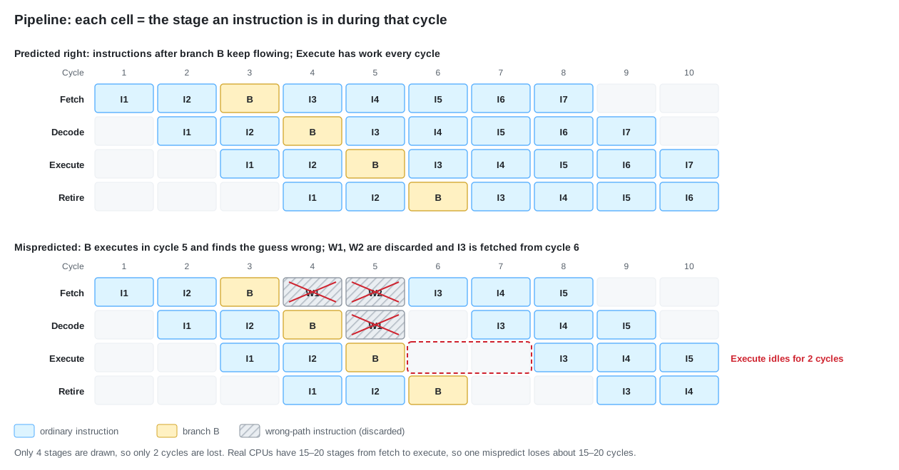
The cost is roughly the pipeline depth from fetch to execute, about 15–20 cycles, about 4–5 ns at 4 GHz. At 4–8 instructions per cycle, that is 60–160 instructions’ worth of execution lost. (Loads issued on the wrong path have already brought lines into the cache, and that is not undone; this is where Spectre-class vulnerabilities come from, not covered here.)
Compare with the numbers in Memory Latency and Bandwidth: an L1 hit is about 1 ns, an L2 hit about 3–5 ns, a branch misprediction about 4–5 ns. One misprediction on the hot path costs about as much as an L2 hit. The difference: a cache miss can overlap with other misses (MLP), while a misprediction throws away the work after it and can’t overlap with it.
1.5 Predictability Comes From the Data: The Sorting Experiment
A classic example (data holds 16384 random integers in 0–199, and the outer loop repeats 10000 times):
for (unsigned i = 0; i < 10000; ++i) {
    for (unsigned c = 0; c < arraySize; ++c) {
        if (data[c] % 2 == 0) {
            evenSum += data[c];
        }
    }
}
Run the same loop with data unsorted and sorted; the sorted version adds a single line, std::sort(data, data + arraySize).
- Unsorted: whether each number is even is completely random, the
ifhas no pattern, and the predictor gets about half right. Each element pays about $0.5 \times (15\text{–}20) \approx 8\text{–}10$ extra cycles on average, several times the loop body itself (1–2 cycles). - Sorted: each value in 0–199 appears about 82 times, so the sorted array alternates in runs: 82 evens, 82 odds, 82 evens… 200 runs in all. The direction changes only at run boundaries, each boundary mispredicts 1–2 times, so a pass of 16384 mispredicts only about 200–400 times, about 1%–2%.
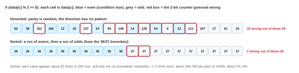
So the sorted run is several times faster (measured later in this section). The lesson: the same branch in the same code is predictable or not depending on the data.
There is a compiler trap here: GCC 13.3 on x86-64 turns this if branch-free from -O1 up. The inner loop has only an and (take the low bit) and a cmove (move the new sum into evenSum only if the condition holds), no conditional jump; -O3 vectorizes it as well. Then sorted and unsorted run at the same speed and the experiment shows nothing. To see the cost of mispredictions you have to add -fno-if-conversion -fno-if-conversion2 -fno-tree-vectorize, which leaves a je in the inner loop. So before arguing about whether there’s a branch, read the assembly. (Why cmov removes a branch and when the compiler won’t use it is in Part 2.)
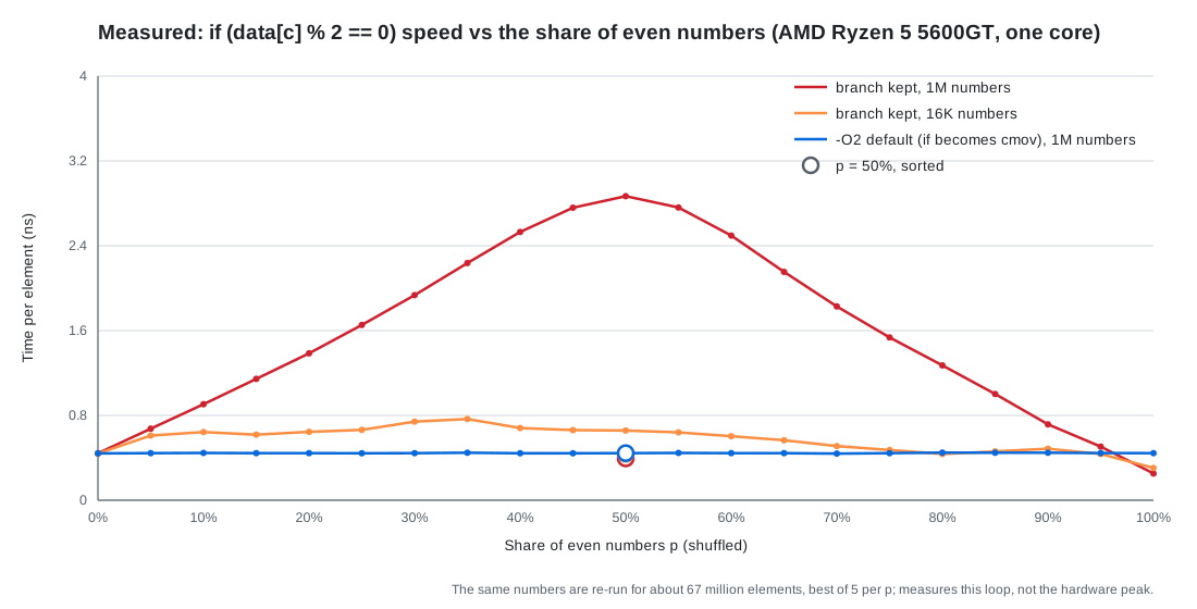
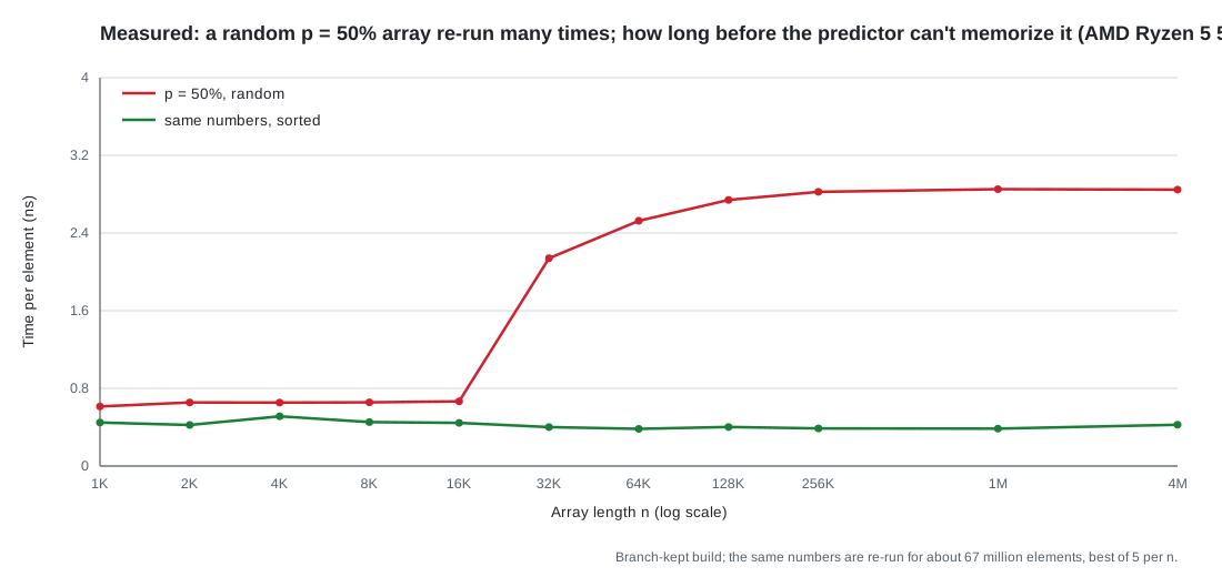
Measured (AMD Ryzen 5 5600GT, one core, GCC 16.2.0,
-O2; the branch-kept build adds-fno-if-conversion -fno-if-conversion2 -fno-tree-vectorize. The share of even numbers p sweeps 0% to 100%, the same numbers are re-run for about 67 million elements, best of 5 per point):
- Branch kept, a million numbers: a tent. At p = 50% it takes about 2.87 ns per element; sorted, about 0.40 ns, about 7 times faster. The curve climbs and falls almost in straight lines: when the direction is random, the best guess is always the majority side, so the misprediction rate is $\min(p, 1-p)$. The extra time per element is about $\min(p, 1-p) \times 4.9\ \text{ns}$: 2.43 ns extra at p = 50%, so about 4.9 ns per mispredict; use it for p = 25% and 0.25 × 4.9 ≈ 1.2 ns, against 1.21 ns measured.
- The
cmovbuild: a flat line at about 0.44 ns per element, regardless of p or sorting. Each element waits for the previous sum (addthencmove, about 2 cycles), and that dependency chain sets its speed.- At the edges, keeping the branch is faster. At p = 100% every guess is right, about 0.25 ns, faster than
cmov; at p = 0% it is about 0.44 ns, because each element jumps twice (over the add, and the loop back edge) and hits the limit of roughly one taken jump per cycle. When to switch tocmovis Part 2.- With only 16384 numbers, the cost almost disappears. Equally random, p = 50% takes only about 0.66 ns, sorted about 0.44 ns, just 1.5 times apart. The same string of 16384 directions is replayed over 4000 times and the predictor memorizes it with its long history. The second chart sweeps the array length at p = 50%: up to 16384 numbers it stays around 0.6–0.7 ns, at 32768 it jumps to about 2.1 ns, and from 260 thousand on it settles at about 2.85 ns. So don’t measure branch costs by replaying a short input over and over: real market data doesn’t repeat, and a replay looks too optimistic.
How to measure: on Linux, perf stat -e branches,branch-misses ./prog gives the number of branches and how many were mispredicted; the ratio is the misprediction rate. Windows has no perf; use AMD uProf on AMD and VTune on Intel. Only a hot-path misprediction rate of several percent or more is worth acting on.
1.6 Branch Kinds: Which Predictor Handles Each
The C++ constructs that produce branches, matched against 1.3:
| Construct | In machine code | Predicted by |
|---|---|---|
if / else, ternary ?:, short-circuit && / ||, loop conditions, break / continue | conditional jump (jcc), fixed target | direction predictor |
| direct function call | call to a fixed address | BTB (unconditional, almost never wrong) |
| function return | ret | RAS |
switch (compiled to a jump table) | indirect jump jmp [table + index×8] | indirect target predictor |
| virtual function, function pointer | indirect call call [register] | indirect target predictor |
A ternary ?: doesn’t necessarily become a jump: the compiler may turn it into a cmov, as in 1.5. Short-circuit evaluation goes the other way: a && b often adds a branch (skip b when a is false).
A virtual call is predictable to the extent that “the actual type at this call site” follows a pattern: if a loop always sees the same type, the target is the same every time and almost never wrong; if types are mixed at random, every call can miss, just like the unsorted case in 1.5.
2. Eliminating Branches: Select, Don’t Guess
Part 1 ended on a puzzle. With a million random numbers, the cmov build sits flat at about 0.44 ns per element, more than 6× faster than the 2.87 ns of the branchy build. Yet when every number is even, the branchy build takes only about 0.25 ns and beats cmov. Removing a branch isn’t free. This part covers what it trades away, the ways to do it, and when the trade pays.
2.1 Control Dependency vs Data Dependency: What Gets Traded
An if in machine code is a conditional jump: which instructions come next depends on the condition. That is a control dependency. As 1.2 showed, the CPU doesn’t wait for it; it guesses a direction and runs ahead. When the guess is right, it doesn’t matter how late the condition is computed. When it’s wrong, the CPU pays about 15–20 cycles.
Eliminating the branch fixes which instructions run, and the condition only decides which value to keep. That is a data dependency: the result is known only once the condition and both candidate values are computed, and the next instruction that uses it has to wait too. There is nothing to guess, so nothing can be mispredicted. But there is also no running ahead, so the condition’s latency is paid every time.
So eliminating a branch trades “an occasional 15–20 cycles” for “1–2 extra cycles every time.” The five techniques below (2.2–2.6) are all this same trade, and 2.7 works out when it pays. All assembly below is real GCC 13.3 -O2 output.
2.2 Ternary and cmov: Prepare Both, Pick One
int pick(int input, int threshold, int value1, int value2) {
    return (input > threshold) ? value1 : value2;
}
GCC emits:
cmpl    %esi, %edi        # compare input with threshold
movl    %edx, %eax        # start with value1
cmovle  %ecx, %eax        # if input <= threshold, replace with value2
ret
cmov (conditional move) is not a jump. It always executes; the flags only decide whether the destination register takes the source value. The front end has nothing to guess and keeps fetching straight ahead.
The compiler does this only when evaluating both sides is safe and cheap:
A side has side effects (a function call, a memory write, I/O): running both sides would change what the program does, so it can’t.
A side reads memory that may not be valid to read:
int load_or_zero(const int* p) {
    return p ? *p : 0;
}
GCC emits
testq %rdi, %rdi+jeand keeps the branch. Acmovwould need to execute*punconditionally, which crashes whenpis null.Both sides are long computations: computing both throws away the work the cheap side would have saved.
The reverse also holds: write an if and the compiler may turn it into cmov on its own. 1.5’s even_sum is one example; the branchy sign in the next section also compiles to setne + cmovg under GCC -O2. A ternary is only more likely to become cmov, not guaranteed. To be sure, read the assembly. Clang has __builtin_unpredictable(cond), which tells the compiler the condition is hard to predict and nudges it toward cmov.
2.3 Branchless Arithmetic: Compute It from Comparisons and Masks
A comparison already yields 0 or 1:
int sign(int x) {
    if (x > 0) return 1;
    if (x < 0) return -1;
    return 0;
}

int sign_branchless(int x) {
    return (x > 0) - (x < 0);   // comparisons yield 0 or 1: positive 1 - 0, negative 0 - 1
}
GCC compiles sign_branchless to setg for x > 0, uses shrl $31 to pull out the sign bit as x < 0, and subtracts. No jump.
Mask select: the mask is all ones when the condition is true and all zeros when it’s false; & and | then assemble the result.
int select_mask(bool cond, int a, int b) {
    int mask = -static_cast<int>(cond);   // 1 -> 0xFFFFFFFF, 0 -> 0
    return (a & mask) | (b & ~mask);      // cond ? a : b
}
The mask has to be all ones or all zeros. ANDing with the bool directly is wrong: 1 & a keeps only the lowest bit of a. To get a mask from the sign, x >> 31 works: all ones for negative values, zero otherwise (C++20 defines signed right shift as arithmetic; before that it was implementation-defined).
1.5’s even_sum without if:
for (unsigned c = 0; c < n; ++c) {
    int x = data[c];
    sum += x & -static_cast<int>((x & 1) == 0);   // add x if even, 0 if odd
}
This compiles to not, and $1, neg, and, add, and the only branch left in the loop is the back edge. As with cmov, every sum waits for those instructions.
It suits numeric code: min/max, clamping. The costs are readability, and the fact that the compiler can usually turn a simple if into cmov by itself. Read the assembly before hand-writing it.
2.4 Lookup Tables: Index, Don’t Branch
A value table: when the input range is small, precompute the result for every input and index with the input at run time.
constexpr int fee_bps[3] = {2, 5, 10};   // fee rates for three order types, in basis points
int fee_lookup(unsigned type) { return fee_bps[type]; }
That compiles to a single movl (%rax,%rdi,4), %eax: truly branchless. The cost becomes one memory access: about 1 ns if the table is in L1D; about 3–5 ns once it spills into L2, already about the price of a mispredict; about 80–120 ns from memory, far worse (see Reference 2.1). Lookup tables only pay when they’re small; a hot-path table needs to stay in L1D.
A function-pointer table:
using HandlerFunc = void(*)(const Order&);
constexpr HandlerFunc handlers[] = {handle_type_0, handle_type_1, handle_type_2};

void process_order(const Order& order) {
    if (order.type < 3) {
        handlers[order.type](order);
    }
}
compiles to:
movl    (%rdi), %eax            # order.type
cmpl    $2, %eax
ja      .L28                    # bounds check: a conditional jump
leaq    handlers(%rip), %rdx
jmp     *(%rdx,%rax,8)          # indirect jump: target read from the table
This doesn’t eliminate the branch. It replaces several conditional jumps with one indirect jump, which the indirect target predictor handles (1.3). When order types follow a pattern (all the same, or a short repeating cycle), it almost never misses; when the types are randomly mixed, it misses often, just like a virtual call. The benefit is that however many types there are, there’s only one jump to predict instead of a chain of ifs. The bounds-check ja is almost never taken and easy to predict.
2.5 if-else Chains and switch: How the Compiler Lays Them Out
An if-else chain: every condition is its own conditional jump. The cost is how many of them run on the way through and how predictable each is: put the most common case first and most passes exit after one or two. Each jump has its own predictor history, so more conditions don’t make each one harder to predict; going deeper just means passing more conditional jumps.
switch: GCC picks one of three layouts depending on how the case values are spread.
Dense cases, each doing something different → jump table:
switch (kind) {
    case 0: handle_type_0(o); break;
    case 1: handle_type_1(o); break;
    // ... case 2, 3, 4
}
cmpl $4, %eax ja .L30 # outside 0–4: jump away leaq .L33(%rip), %rdx # .L33 is a table of relative addresses of each case's code movslq (%rdx,%rax,4), %rax addq %rdx, %rax notrack jmp *%rax # indirect jumpLike the function-pointer table, it’s one indirect jump. The lookup cost doesn’t depend on the number of cases, but whether it’s predicted well still depends on whether
kindhas a pattern.Dense cases, each only returning a value → value table:
switch (type) {
    case 0: return 2;
    case 1: return 5;
    // ... case 2, 3, 4
    default: return 0;
}
GCC emits a constant array (named
CSWTCHin the assembly) and reads it with onemovl (%rax,%rdi,4), %eax, leaving only an easy bounds check. This one is truly branchless.Sparse cases (1, 10, 1000) → a chain of compares:
cmpl $10+je,cmpl $1000+je, and acmovnefor the last one. With many cases it becomes a binary-search tree of compares.
So “make the cases dense” helps, but what it buys is a jump table or a value table. The first still has to be predicted; only the second removes the branch.
2.6 Loop Unrolling: Fewer Back Edges, but the Win Isn’t in Branches
One iteration does the work of several:
long long sum_unroll4(const int* a, unsigned n) {
    long long s0 = 0, s1 = 0, s2 = 0, s3 = 0;
    unsigned i = 0;
    for (; i + 4 <= n; i += 4) {
        s0 += a[i];
        s1 += a[i + 1];
        s2 += a[i + 2];
        s3 += a[i + 3];
    }
    for (; i < n; ++i) s0 += a[i];   // fewer than 4 left
    return s0 + s1 + s2 + s3;
}
What it saves on branches: one back edge per 4 elements. But as 1.3 showed, a loop’s back edge is almost never mispredicted anyway, so unrolling mainly saves the i++, cmp, jne instructions themselves, not mispredicts. If the body has a hard-to-predict if, unrolling turns it into 4 of them; not one goes away.
The real win: the four accumulators s0–s3 are four independent dependency chains that run in parallel (the multiple accumulators from #2), which has nothing to do with branches.
- A short fixed-count loop like 4 iterations is fully unrolled by GCC
-O2already; no need to do it by hand. - To ask the compiler to unroll: GCC uses
#pragma GCC unroll 4;#pragma unrollis Clang’s spelling. - More unrolling means more code, which competes for L1I and the uop cache. On a hot path, more is not always better.
2.7 Branchless Isn’t Always Faster: How to Decide
Start with even_sum’s dependency chain per element:
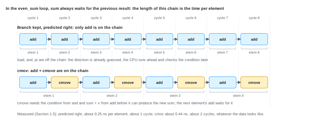
Every sum waits for the previous one. With the branch kept and predicted right, only one add sits on the chain, about 1 cycle; the and and je that test parity are off the chain and checked later. With cmov, the chain is add then cmove, and cmove also waits for the condition: about 2 cycles. 1.5’s measurements line up: at p = 100% the branchy build takes about 0.25 ns per element and cmov about 0.44 ns; sorted, the branchy build takes about 0.40 ns, also faster than cmov.
When to switch: compare what each side adds per element.
$$ \underbrace{\text{miss rate} \times \text{cost of one mispredict}}_{\text{extra for the branch}} \quad\text{vs}\quad \underbrace{\text{extra per element for cmov}}_{\approx\, 0.44 - 0.25 = 0.19\ \text{ns}} $$One mispredict costs about 4.9 ns, so for this loop the break-even miss rate is about $0.19 / 4.9 \approx 4\%$: below about 4% keep the branch, above about 4% switch to cmov. In the measurements, at p = 95% (about 5% misses) the branchy build is already at about 0.51 ns, slower than cmov; at p = 100% it’s about 0.25 ns, faster. That 4% belongs to this loop only: what cmov adds depends on what it puts on the chain, so another loop needs its own arithmetic.
Example: binary search over a large array, where cmov can be slower. Each level of a binary search reads one middle element and compares it to decide left or right:
const int* lower_bound_cmov(const int* base, std::size_t n, int key) {
    while (n > 1) {
        std::size_t half = n / 2;
        base = (base[half] < key) ? base + half : base;   // cmov: the next address waits for base[half] to arrive
        n -= half;
    }
    return base + (*base < key);
}
GCC -O2 compiles the middle line to cmpl (%rcx), %edx + cmovg; an if compiles the same way, and keeping the branch takes -fno-if-conversion. The keys are random, so each level goes left or right half the time, and the branchy version mispredicts about 50% per level.
By the arithmetic above, 50% is far above 4%, so switch to cmov. For a small array that’s right; for a large one it can flip. The difference is which address the next level reads, and when that becomes known:
- The
cmovversion: the nextbaseis the result ofcmovg, andcmovgwaits forbase[half]to arrive. So the next level’s read can’t be issued until this level’s read comes back. The levels queue up one after another, each paying a full read latency. - The branchy version: the CPU doesn’t wait for
base[half]. It guesses a side, computes the next level’s address, and issues that read right away, so two reads are in flight together (memory-level parallelism). Guess right and the next level’s data arrives about when this level’s does, saving a whole read latency. Guess wrong and the early read is wasted; the pipeline flush costs about 5 ns and the correct address is read again: as slow ascmov, plus those 5 ns.
So which wins depends on how long one read takes:
- Array in L1 or L2: a read takes about 1–5 ns. That’s all a right guess saves, while a wrong guess costs about 5 ns each time, and half the guesses are wrong.
cmovwins. - The last levels read memory: a read takes about 80–120 ns. A wrong guess adds only about 5 ns; a right one saves about 100 ns. The branchy version wins.
The figure shows how the three versions schedule their reads when the last 6 levels all go to memory:
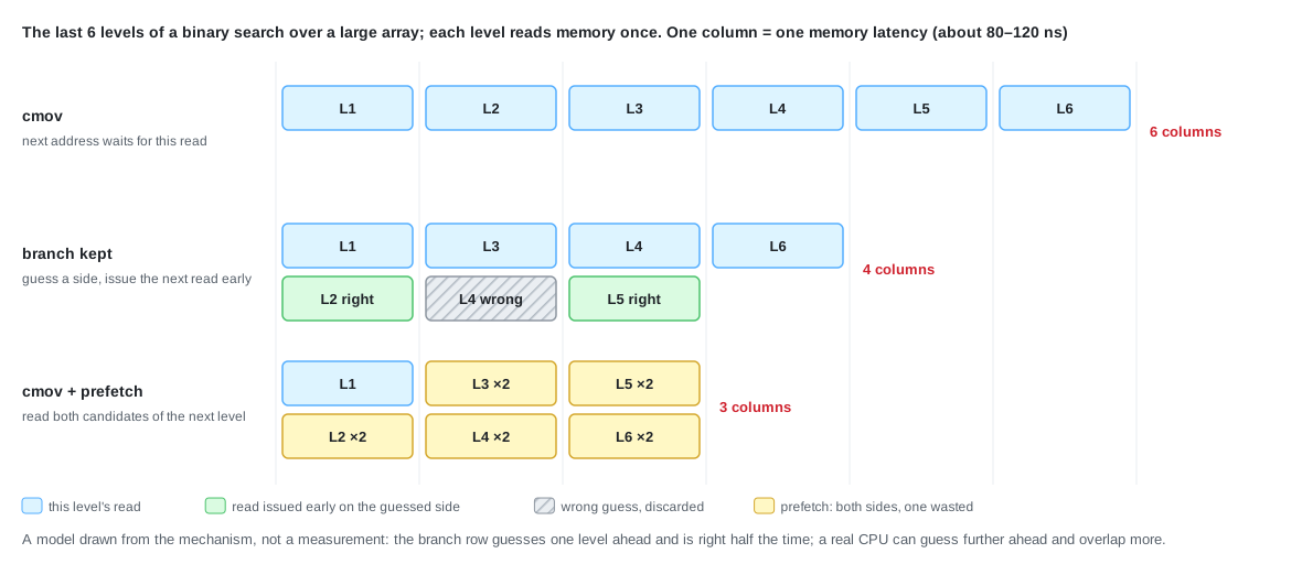
In the figure’s model (guess one level ahead, right half the time), cmov waits one memory latency per level; the branchy version resolves 1.5 levels per round trip on average, about 2/3 of a latency per level. For a 1 GiB int array: $2^{28}$ elements, 28 levels. Over repeated searches the top levels keep reading the same few elements, which stay in cache: a 16 MiB L3 holds about 260K cache lines, so roughly the first 18 levels ($2^{18} \approx$ 260K elements) stay cached and the last ~10 read memory. cmov takes about $10 \times 100 = 1000$ ns per search; the branchy version about $10 \times 67 + 28 \times 50\% \times 5 \approx 740$ ns. That’s a model estimate, not a measurement; a real CPU guesses more than one level ahead and can overlap even more.
Getting both: cmov + prefetch. Don’t guess; read both candidates of the next level early:
const int* lower_bound_prefetch(const int* base, std::size_t n, int key) {
    while (n > 1) {
        std::size_t half = n / 2;
        n -= half;
        __builtin_prefetch(base + n / 2);          // read if the next level goes left
        __builtin_prefetch(base + half + n / 2);   // read if the next level goes right
        base = (base[half] < key) ? base + half : base;
    }
    return base + (*base < key);
}
__builtin_prefetch only tells the hardware “this address is needed soon, pull it into cache”; it doesn’t wait for the result and doesn’t fault on a bad address. The next level is always one of the two, so nothing is mispredicted, and each memory latency resolves 2 levels (the figure’s third row). The cost is that half the prefetches are wasted, doubling the bandwidth used.
How to decide:
- Read the assembly and confirm the branch is really there: the compiler may already have turned it into
cmov, or turned your ternary back into a branch. - Measure the miss rate with
perf stat -e branches,branch-misses. Below a few percent, keep the branch. - If the miss rate is high and the branch is on the critical path, switch to
cmov, a mask, or a table, then measure again.
3. Hints and Separation: Tell the Compiler Which Side Is Common, Move the Rare Side Away
Branch optimization can be ordered in three steps: eliminate, then predict, then separate. Part 2 was elimination. For the branches that can’t be eliminated and have to stay, what’s left is to lay the common side out as a straight line and move the rare side far away. And whatever can be decided at compile time shouldn’t wait until run time. Everything in this part changes how the compiler lays out code, not the CPU’s predictor. All assembly below is GCC 13.3 -O2 output.
3.1 Branch Hints: They Change Layout, Not the Predictor
#define LIKELY(x) __builtin_expect(!!(x), 1)     // !! turns x into 0 or 1
#define UNLIKELY(x) __builtin_expect(!!(x), 0)

int process(const int* q, int n) {
    if (UNLIKELY(n <= 0)) {    // C++20 can also write if (n <= 0) [[unlikely]] {
        report_error(n);
        return -1;
    }
    return q[0] + q[n - 1];
}
On the left of the figure is the machine code for this version; on the right, the hint deliberately reversed to LIKELY(n <= 0):
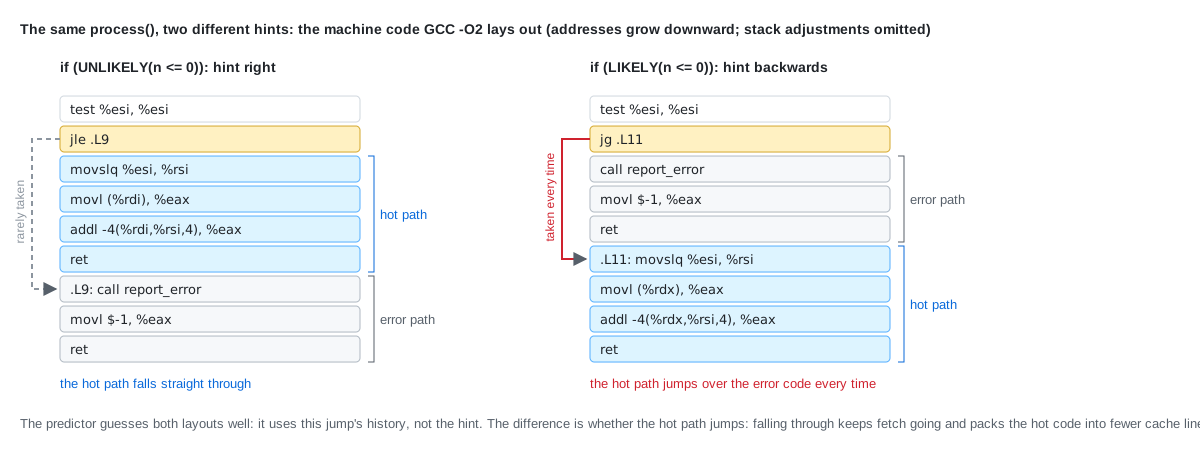
The instructions are almost identical; only the order differs:
- Hint right:
jle .L9jumps only on error, the hot path’s 4 instructions follow it directly and fall through toret; the error handling goes at the end. - Hint reversed: the error handling follows the test, and the hot path is reached by
jg .L11, taken every time.
There is no “hint bit” in the machine code: __builtin_expect is only for the compiler, and the CPU just sees ordinary jle and jg. At run time the predictor still guesses from this jump’s history, and it predicts both layouts well. So why is falling through better?
- Taken jumps break up fetch: a taken branch makes fetch restart at a new address; that’s the “about one taken jump per cycle” limit in 1.5’s measurements. A hot path that doesn’t jump keeps fetch going straight ahead.
- Hot code packs together: the hot path’s instructions form one contiguous run, using fewer L1I cache lines and uop-cache entries, with no rare error code in the middle.
- With no predictor record, the fall-through side is the “right guess”: when the predictor has no record of this jump (first execution, or it hasn’t run for a while and the record was evicted), fetch doesn’t even know there’s a jump here and simply keeps fetching sequentially, which amounts to guessing “not taken.” With the hot path on the fall-through side, a cold start doesn’t mispredict either. A trading system’s order path runs rarely, so this point matters most.
The compiler guesses too: without any hint, GCC has its own heuristics. Replace the error handling with a printf and write no hint at all, and GCC lays it out the same as the left side (the side that calls a function and returns a negative constant is treated as rare). Hints only help when the compiler’s guess is wrong. Also, a strongly biased condition makes the compiler more likely to keep a branch instead of turning it into cmov.
The cost of a backwards hint: the hot path takes an extra jump every time, and the hot code is split by the error handling. It doesn’t add mispredicts in steady state, but every pass is a bit slower, and a cold start mispredicts. So write hints to match the real probabilities; if unsure, don’t write them, or leave it to PGO (3.3).
Other hints:
[[assume(expr)]](C++23, supported by GCC 13): tells the compilerexpralways holds, so it can drop checks based on it. If it’s wrong, the behavior is undefined. It’s equivalent toif (!(expr)) __builtin_unreachable();.[[noreturn]]: the function never returns (likestd::abort). GCC treats the path leading to it as rare.noexceptisn’t a branch hint: it promises the function won’t throw, so the compiler can drop exception-handling paths, and the standard library (e.g.std::vectorgrowth) uses it to move instead of copy. That’s why low-latency code often uses error codes instead of exceptions.
3.2 Hot/Cold Splitting: Move the Rare Path Out
Pull the rare path into its own function and mark it cold and noinline:
__attribute__((noinline, cold))
void handle_slow_path(const Packet& pkt) {
    // handle the error, log, drop the packet...
}

void process_packet_refactored(const Packet& pkt) {
    if (!pkt.is_valid() || pkt.type != MsgType::TRADE) {
        return handle_slow_path(pkt);   // the slow path is a single call
    }
    // everything left is the fast path, a straight line
}
It compiles to:
        .text
process_packet_refactored:
        movslq  4(%rdi), %rax
        testl   %eax, %eax
        jle     .L3                     # invalid packet: jump to the cold area
        cmpl    $1, (%rdi)
        jne     .L3                     # not a trade: jump to the cold area
        addq    %rax, g_traded(%rip)    # fast path
        ret

        .section .text.unlikely         # cold area: placed apart from hot code
process_packet_refactored.cold:
.L3:    jmp     handle_slow_path
handle_slow_path:                       # the cold function lives entirely here
        ...
Three things happened:
handle_slow_pathgoes entirely into the.text.unlikelysection. The linker groups all.text.unlikelytogether, far from hot code.coldalso makes the compiler treat the path that calls it as rare: without anyUNLIKELY, GCC split the jump to the slow path intoprocess_packet_refactored.coldand put it in the cold area too.noinlinekeeps the slow path from being inlined back. Inlined into the hot function, it would bloat it and might force extra register saves, slowing the hot path down.
The hot function is left with 7 instructions, so L1I and the uop cache hold only code that actually runs. Conversely, __attribute__((hot)) puts a function in .text.hot, next to the other hot functions.
3.3 PGO: Measured Statistics Instead of Hand-Written Hints
PGO (profile-guided optimization) takes three steps:
g++ -O2 -fprofile-generate main.cpp -o app   # 1. instrumented build: counters on every branch and function
./app <representative input>                 # 2. run it; counts are written to .gcda files
g++ -O2 -fprofile-use main.cpp -o app        # 3. rebuild using the counts
In step 3 the compiler knows the real taken ratio of every branch, so it does what 3.1 and 3.2 did by hand: which side falls through, which functions are cold, whether to inline, whether to use cmov. It beats hand-written hints because the numbers are measured.
The trap in trading systems: PGO only knows what ran during training. A trading system spends most of its time receiving market data and updating state; the path that actually sends an order runs rarely. If the training run sends few or no orders, the order path is treated as cold code. A small program to try it:
void on_quote(const Quote& q, double threshold) {
    g_fair = g_fair * 0.99 + (q.bid + q.ask) * 0.005;
    double edge = g_fair - q.ask;
    if (edge > threshold) send_order(q, edge);   // rarely true on real market data
}
| During training | Where send_order goes | The calling code in on_quote |
|---|---|---|
| No orders at all | .text.unlikely | split into on_quote.cold, in the cold area |
| An order on every quote (simulated dummy execution) | .text.hot | stays in the hot area |
No orders, with -fprofile-partial-training | .text.hot | stays in the hot area, no cold part |
The most important path ends up in the coldest place, and on a cold start it also mispredicts because it isn’t on the fall-through side. GCC’s documentation also says functions never executed in training are optimized for size, as with -Os (this small function shows no difference; only its placement changed). Two fixes:
- Dummy execution: in a test mode, run the order path on every quote without actually sending the order. The profile then counts it as hot.
-fprofile-partial-training(GCC 10 and later): code that didn’t run during training is optimized normally instead of being moved to the cold area.
The stages before the order path that run on every quote (parsing, updating the book, computing signals) run plenty during training, and PGO still helps them.
3.4 Compile-Time Branches: The Condition Is Settled at Compile Time
There are four forms, grouped by what they choose: if constexpr picks a block of code inside a function, enable_if and requires pick one function among overloads, and std::conditional_t picks a type. In every case the condition has to be known at compile time.
3.4.1 if constexpr: Pick One Branch at Compile Time, Don’t Instantiate the Other
What it is: since C++17, the condition of if constexpr (cond) must be a compile-time constant. The compiler picks a branch at compile time and discards the other one without instantiating it.
template <typename T>
std::size_t get_size(const T& t) {
    if constexpr (requires { t.size(); }) return t.size();   // discarded when T is int
    else return 0;
}
get_size(std::string("hello")) returns 5 and get_size(42) returns 0.
How it differs from a plain if: not at run time. When the condition is a compile-time constant, a plain if leaves no branch under -O2 either:
template <typename T> int k() { if (std::is_integral_v<T>) return 1; else return 2; }
int kk() { return k<int>(); }   // GCC -O2: movl $1, %eax; ret
The difference is whether it compiles. Both branches of a plain if are instantiated, so both must be valid for this T. Replace the if constexpr above with if (std::is_class_v<T>) return t.size(); and it fails to compile when T is int (GCC: request for member 'size' in 't', which is of non-class type 'const int'), even though that branch would never run.
When to use it: inside one template, when different types need different code and some of that code is only valid for some types.
3.4.2 std::enable_if: If the Condition Fails, the Overload Doesn’t Exist
What it is: if constexpr branches inside one function; enable_if chooses among several overloads. std::enable_if_t<cond, Type> is Type when the condition holds and undefined otherwise. Use it in a template’s signature and, when the condition fails, the signature is ill-formed and the compiler quietly drops that overload from the candidates. The rule is called SFINAE (substitution failure is not an error).
How to write it: in the template parameter list, make it a non-type template parameter (type int, default 0):
template <typename T, std::enable_if_t<std::is_integral_v<T>, int> = 0>
void print(T value) { std::cout << "integral: " << value << std::endl; }

template <typename T, std::enable_if_t<!std::is_integral_v<T>, int> = 0>
void print(T value) { std::cout << "non-integral: " << value << std::endl; }
print(1) takes the first and print(2.5) the second.
The common mistake: writing it as a default template argument, typename = std::enable_if_t<…>. Default arguments aren’t part of the signature, so both templates have the same signature and GCC reports redefinition.
3.4.3 requires and Concepts: The C++20 Way
What it is: since C++20 a constraint goes straight after requires, without borrowing the return type or a template parameter:
template <typename T> requires std::is_integral_v<T>
void print20(T value) { std::cout << "integral: " << value << std::endl; }

template <typename T>
void print20(T value) { std::cout << "non-integral: " << value << std::endl; }
When both match (say, int), the constrained one is more specialized and wins; double matches only the second. A concept gives a set of constraints a name, e.g. template <Arithmetic T> T add(T a, T b). Prefer this in new code: it reads better than enable_if and gives clearer errors.
3.4.4 std::conditional_t: Pick a Type at Compile Time
What it is: the first three choose code; std::conditional_t<cond, A, B> chooses a type: A if the condition holds, B otherwise.
enum class QueueMode { Blocking, NonBlocking };
struct BlockingQueue { /* sleeps when empty */ };
struct SpinQueue { /* busy-waits when empty */ };

template <QueueMode Mode>
using Queue = std::conditional_t<Mode == QueueMode::Blocking, BlockingQueue, SpinQueue>;
In a trading system: all four say the same thing: configuration that can be fixed at compile time belongs in a template parameter. “Blocking or not” written as a run-time if (config.blocking) reads the config and tests it on every message; as a template parameter, only the chosen code exists in the binary.
3.5 Semi-Static Branches: When the Switch Rarely Changes, Stop Testing It
3.5.1 The Setup: A Switch That Changes Once an Hour
Say you’re writing a trading loop fed a million quotes per second. The code has a test like this:
for (...) {
    if (use_strategy_a) {
        handle_a(x);   // strategy A
    } else {
        handle_b(x);   // strategy B
    }
}
use_strategy_a is a switch (say, a risk flag) that changes once an hour: true for the first 3600 seconds, and only at second 3601, when risk control trips, does it become false. Yet for every quote the loop loads it, compares it and jumps on the result: 3.6 billion times an hour, almost always with the same answer.
First, what is not slow: with the switch staying true, the if goes the same way every time, so the predictor is right almost every time and misses only once, at second 3601. The problem isn’t mispredicts; it’s two small things:
- A few instructions every time: load, compare, conditional jump, 3.6 billion times for an answer already known.
- The first pass after a long idle stretch: if the hot path doesn’t run continuously but only every few minutes, other code runs in between and the predictor’s record of this
ifmay be evicted. When execution gets here again, the predictor can only guess blindly, and a wrong guess costs 15–20 cycles.
3.5.2 The Simplest Fix: Move the Test Out of the Loop
If the switch doesn’t change during a run of the loop, test it once before the loop and write two loops (loop unswitching):
if (use_strategy_a) {
    for (int i = 0; i < n; ++i) handle_a(xs[i]);
} else {
    for (int i = 0; i < n; ++i) handle_b(xs[i]);
}
The test goes from once per quote to once per run of the loop, and the loop body has no test at all. When the switch is something like a function parameter that can’t change inside the loop, GCC 13 -O2 makes this split by itself.
When it can’t be moved out: a real trading loop is an event loop that never stops, and the switch is changed by another thread (risk control) at any moment. Then the loop has to re-read the switch every time: it may change at any moment, and a copy hoisted outside would never see the change. When the switch is a global and the loop calls other functions, the compiler won’t split it for you either. This case, “rarely changes, but may change at any moment,” is where semi-static branches come in.
3.5.3 How a Semi-Static Branch Works: Hard-Code the Target, Rewrite the Instruction to Switch
BranchChanger ch(handle_a, handle_b);
void refresh_strategy(bool use_a) {
  ch.set_direction(use_a);  // risk thread: rewrite the jump to go to handle_a or handle_b
}
for (...) {
  ch.branch(x);             // hot path: no test, just jump
}
(Schematic code from the maxlucuta/semi-static-conditions library.) Three steps:
ch.branchcontains one jump: it’s a tiny function made of a single instruction (a stub), and that instruction says “jump to handle_a, unconditionally.” The hot path calls it and lands in the strategy without loading or testing anything.- The target address is inside the instruction: this x86
jmpis 5 bytes; the first byte means “jump” (0xE9) and the other 4 are the target (strictly, how far it is from the current position). - Switching strategy means rewriting those 4 bytes: at second 3601, when risk control trips,
set_directionmemcpys handle_b’s position into them. A program rewriting its own instructions at run time is self-modifying code (SMC).
Against the two small things in 3.5.1: no quote loads or compares the switch any more; and since the target is in the instruction, even if the predictor remembers nothing, the CPU knows where to go as soon as it reads the instruction, losing only a few cycles.
3.5.4 The Costs: Switching Is Expensive and Not Very Safe
- One switch costs over a hundred cycles: the CPU may already have fetched the old jump into the pipeline. Once the instruction changes, it has to throw all of that away and fetch again. So
set_directioncan only be called occasionally; once an hour is fine. - The code’s memory has to be writable: normal program code is read-only, and “writable memory isn’t executable” (W^X) is a basic security rule that exists precisely to stop anyone writing into code. By default this library keeps the code readable, writable and executable; the safe mode opens write permission only around each rewrite, which makes
set_directionslower still. - Threads need care: while the risk thread rewrites the instruction, the trading thread may be executing it. Also, usually only one
BranchChangeris allowed per function signature.
So the order is: move the test out of the loop if you can; only if you can’t, the hot path runs rarely, and those few cycles matter, consider a semi-static branch.
3.6 Compile-Time Decision Trees: Composable Like Building Blocks, as Fast as Hand-Written ifs
The bottom line first: this isn’t a branch optimization. It compiles to the same thing as hand-written nested ifs, with every test still there. It solves a different problem: strategies you want to assemble like building blocks and re-parameterize, without paying for that flexibility at run time. To see that, compare three ways of writing the same strategy.
3.6.1 One Strategy, Three Ways to Write It
The strategy itself is simple:
- Position above 100: close out (CLOSE).
- Otherwise, volatility above 0.5: do nothing (NONE).
- Otherwise look at order-book imbalance (OBI): above 0.2 buy (BUY), above -0.2 do nothing, else sell (SELL).
Version 1: hand-written nested ifs. The most direct, and the fastest:
ActionType decide_hand(const MarketContext& c) {
    if (std::abs(c.position) >= 100) return ActionType::CLOSE;
    if (c.volatility > 0.5) return ActionType::NONE;
    if (c.obi > 0.2) return ActionType::BUY;
    if (c.obi > -0.2) return ActionType::NONE;
    return ActionType::SELL;
}
The trouble is maintenance: with a dozen instruments each using its own thresholds, or with the “momentum” part reused across several strategies, these ifs get copied many times, each copy with its own numbers.
Version 2: a tree assembled at run time from virtual functions. To make strategies composable and reusable, a common approach is to make every node an object:
struct Node {
    virtual ~Node() = default;
    virtual ActionType evaluate(const MarketContext& ctx) const = 0;
};
struct Decision : Node {
    bool (*check)(const MarketContext&);   // this node's condition
    std::unique_ptr<Node> left, right;     // left if the condition holds, right otherwise
    ActionType evaluate(const MarketContext& ctx) const override {
        return check(ctx) ? left->evaluate(ctx) : right->evaluate(ctx);
    }
};
(A Leaf node that just returns an action is omitted.) The tree can be read from a config file and assembled, even swapped during the trading day. The cost is at every level: calling check is an indirect call through a function pointer, calling the child is a virtual call, another indirect call, and the child pointer has to be loaded first, from nodes scattered on the heap that may miss in cache. The compiler can’t see through these pointers, so it can’t inline anything or merge the compares. How virtual functions are implemented and what they cost: Virtual Functions in the Reference.
Version 3: a compile-time decision tree. Replace version 2’s node objects with types, and the tree is assembled at compile time:
template<typename Cond, typename Left, typename Right>
struct DecisionNode {
    HFT_FORCE_INLINE static ActionType evaluate(const MarketContext& ctx) {
        if (HFT_LIKELY(Cond::check(ctx))) return Left::evaluate(ctx);
        return Right::evaluate(ctx);
    }
};

using ExampleStrategy = DecisionNode<
    IsPositionSafe<100>,                 // |position| < 100 ?
    DecisionNode<
        IsHighVol<500>,                  // volatility > 0.5 ?
        ActionNode<ActionType::NONE>,
        MomentumBlock<200>               // OBI > 0.2 buy, OBI > -0.2 hold, else sell
    >,
    ActionNode<ActionType::CLOSE>
>;
ActionNode<A> is a leaf that returns an action; conditions like IsHighVol<500> are types with a threshold parameter and a static bool check(ctx); MomentumBlock<200> is a small pre-assembled subtree whose threshold is a parameter; HFT_LIKELY is __builtin_expect(!!(x), 1) and HFT_FORCE_INLINE forces inlining. It’s assembled from blocks just like version 2, but every node knows its children at compile time and every evaluate is a static function, so everything inlines all the way down.
3.6.2 What the Three Versions Compile To
GCC 13.3 -O2:
| Cost per decision | Composable, reusable? | Changing the strategy | |
|---|---|---|---|
Hand-written if | 3 conditional jumps + 1 setbe | No; variants are copied and edited | Recompile |
| Run-time virtual tree | 2 indirect calls + a child-pointer load per level | Yes | Change the config, even at run time |
| Compile-time tree | 3 conditional jumps + 1 setbe, same as hand-written | Yes | Recompile |
The compile-time tree and the hand-written ifs compile to nearly identical instructions (only the order differs, because every level of the tree carries HFT_LIKELY): std::abs(position) < 100 becomes one unsigned compare, and the last node becomes a branchless setbe. The tests remain, because they look at market data that’s only known at run time; whether each branch is predictable still depends on whether the data has a pattern (1.5).
So its relation to virtual functions is this: it replaces version 2. It’s no faster than hand-written ifs; it’s faster than the run-time tree while keeping the run-time tree’s composability. Put another way: the run-time tree is dynamic polymorphism (virtual functions, choosing the function by the object at run time), and the compile-time tree is static polymorphism (templates, choosing the function by the type at compile time). It’s the same trade as replacing virtual functions with CRTP: inlining and speed in exchange for a structure fixed at compile time.
3.6.3 When to Use It, and When Not
Useful: when a strategy has many variants sharing the same blocks, and the structure and thresholds are fixed before deployment (parameters tuned offline, then compiled and shipped). For example, a dozen instruments running the same logic with different thresholds:
using BtcStrategy = DecisionNode<IsPositionSafe<100>, MomentumBlock<200>, ActionNode<ActionType::CLOSE>>;
using EthStrategy = DecisionNode<IsPositionSafe<50>,  MomentumBlock<350>, ActionNode<ActionType::CLOSE>>;
Each is one type definition, and each compiles as fast as hand-written code. By hand, it would be a dozen nearly identical copies of the ifs.
Not useful:
- Only one strategy: write the
ifs by hand; it reads better. - The strategy’s structure must change during the trading day: only a run-time tree can do that. If only the thresholds change and the structure stays, make the thresholds ordinary member variables and keep the structure as a compile-time tree; each test then costs one extra memory read.
3.6.4 Watch Out
- Every node uses
HFT_LIKELY, which assumes every condition is usually true and the left side is common. That’s fine forIsPositionSafe; but ifIsHighVolis usually false, the hint here is backwards (the cost in 3.1). Write hints per node from the real probabilities, or leave it to PGO. - Changing the strategy means recompiling; a deep tree costs compile time and code size, and template errors are hard to read.
In Practice
The hot/cold splitting of 3.2 matches the B8 Unmarked Cold Path card below: which calls count as cold, how to mark them, how to confirm.
- Signal: a hot function calls functions only on rare branches, such as error and logging functions, asserts, one-time initialization, or calls inside
if (ret < 0)or aswitch’sdefault.- What counts as cold: the branch at the call site is taken less than about 0.1% of the time.
- Cause: cold code sits between hot code in source order and takes up instruction cache; the compiler also cannot lay out the branch as “almost never taken”.
- Fix: put
[[gnu::cold]]on the called function’s definition (__attribute__((cold))for older standards and C); on the declaration alone it does nothing. Error functions called from a cold function must be marked too; it does not propagate.- The caller is what benefits: the cold function itself is no faster; the hot function’s instructions get more compact.
- Verify:
- first confirm the branch really is cold: Intel’s
branchprob.pymeasures each branch’s actual taken rate with PMU events; with no workload to run,gccbranchprob.pyparses GCC’s compile-time static estimate (-fdump-tree-profile_estimate-lineno);- then check with
-O2 -Sthat the cold function has moved after the hot function’sret.- Mechanism: #7 3.2 Hot/Cold Splitting.